KEY CONCEPTS & TECHNIQUES IN GIS Part 5 doc
Bạn đang xem bản rút gọn của tài liệu. Xem và tải ngay bản đầy đủ của tài liệu tại đây (181.42 KB, 13 trang )
40 KEY CONCEPTS AND TECHNIQUES IN GIS
6.2 Spatial Boolean logic
In Chapter 4, we looked briefly at Boolean logic as the foundation for general com-
puting. You may recall that the three basic Boolean operators were NOT, AND and
OR. In Chapter 4, we used them to form query strings to retrieve records from attrib-
ute tables. The same operators are also applicable to the combination of geometries;
and in the same way that the use of these operators resulted in very different outputs,
the application of NOT, AND and OR has completely different effects on the com-
bination (or overlay) of layer geometries.
Figure 26 illustrates the effect of the different operands in a single overlay opera-
tion. This is why we referred to overlay as a group of functions. Figure 26 is possi-
bly the most important in this book. It is not entirely easy to digest the information
provided here and the reader is invited to spend some time studying each of the sit-
uations depicted. Again, for pedagogical reasons, there are only two layers with only
one feature each. In reality, the calculations are repeated thousands of times when
we overlay two geographic datasets. What is depicted here is the resulting geometry
only. As in the example of Figure 23 above, all the attributes from all the input
layers are passed on to the output layer.
Depending on whether we use one or two Boolean operators and how we relate
them to the operands, we get six very different outcomes. Clearly one overlay is not
the same as the other. At the risk of sounding overbearing, this really is a very impor-
tant figure to study. GIS analysis is dependent on the user understanding what is
All but A and B
Everything not A or B Separate identities
for each segment
Any A that does
not include B
Union levels A not B
Intersect A and B
Coincidence A and B A or B but not both Any part A or B
Not intersect Union A or B
A
+
B
Figure 26 Spatial Boolean logic
Albrecht-3572-Ch-06.qxd 7/13/2007 5:08 PM Page 40
COMBINING SPATIAL DATA 41
happening here and being able to instruct whatever system is employed to perform
the correct overlay operation.
The relative success of the overlay operations can be attributed to their cognitive
consonance with the way we detect spatial patterns. Overlays are instrumental in
answering questions like ‘What else can be observed at this location?’, or ‘How often
do we find woods and bison at the same place?’.
6.3 Buffers
Compared to overlay, the buffer operation is more quantitative if not analytical. And
while, at least in a raster-based system, we could conceive of overlay as a pure data-
base operation, buffering is as spatial as it gets. Typically, a buffer operation creates
a new area around our object of interest – although we will see exotic exceptions
from this rule. The buffer operation takes two parameters: a buffer distance and
the object around which the buffer is to be created. The result can be observed in
Figure 27.
A classical, though not GIS-based, example of a buffer operation can be found in
every larger furniture store. You will invariably find some stylized or real topo-
graphic map with concentric rings usually drawn with a felt pen that center on the
location of the store or their storage facility. The rings mark the price that the store
charges for the delivery of their furniture. It is crude but surprisingly functional.
Regardless of the dimension of the input feature class (point, line or polygon), the
result of a regular buffer operation is always an area. Sample applications for points
would be no-fly zones around nuclear power plants, and for lines noise buffers
around highways. The buffer distance is usually applied to the outer boundary of the
object to be buffered. If features are closer to each other than the buffer distance
between them, then the newly created buffer areas merge – as can be seen for the
two right-most groups of points in Figure 27.
There are a few interesting exceptions to the general idea of buffers. One is the
notion of inward buffers, which by its nature can only be applied to one- or higher-
dimensional features. A practical example would be to define the core of an ecological
Original Points Buffered Points Dissolved Buffers
Figure 27 The buffer operation in principle
Albrecht-3572-Ch-06.qxd 7/13/2007 5:08 PM Page 41
42 KEY CONCEPTS AND TECHNIQUES IN GIS
reserve (see Figure 28). A combination of the regular and the inverse buffer applied
simultaneously to all features of interest is called a corridor function (see Figure 29).
Finally, within a street network, the buffer operation can be applied along the edges
(a one-dimensional buffer) rather than the often applied but useless as-the-crow-flies
circular buffer. We will revisit this in the next chapter.
Core
Figure 28 Inward or inverse buffer
Figure 29 Corridor function
Albrecht-3572-Ch-06.qxd 7/13/2007 5:08 PM Page 42
COMBINING SPATIAL DATA 43
6.4 Buffering in spatial search
A few paragraphs above we saw how overlay underlies some of the (not overtly)
more complicated spatial search operations. The same holds true for buffering.
Conceptually, buffers are in this case used as a form of neighborhood. ‘Find all
customers within ZIP code 123’ is an overlay operation, but ‘Find all customers in a
radius of 5 miles’ is a buffer operation. Buffers are often used as an intermediate
select, where we use the result of the buffer operation in subsequent analysis (see
next section).
6.5 Combining operations
If the above statement that buffers and overlays make up in practice some 75% of
all analytical GIS functionality is true, then how is it that GIS has become such an
important genre of software? The solution to this paradox lies in the fact that opera-
tions can be concatenated to form workflows. The following is an example from a
major flood in Mozambique in 2000 (see Figure 30).
Input layers
Roads Towns River
Directly affected;
under water
Indirectly affected;
dry but cut off
Not affected at all
Overlay and buffer
Overlay
Identification of
indirectly affected
towns
Figure 30 Surprise effects of buffering affecting towns outside a flood zone
Albrecht-3572-Ch-06.qxd 7/13/2007 5:08 PM Page 43
44 KEY CONCEPTS AND TECHNIQUES IN GIS
We start out with three input layers – towns, roads and hydrology. The first step
is to buffer the hydrology layer to identify flood zones (this makes sense only in
coastal plains, such as was the case with the Southern African floods in 2000). Step
two is to overlay the township layer with the flood layer to identify those towns that
are directly affected. Parallel to this, an overlay of the roads layer with the flood
layer selects those roads that have become impassable. A final overlay of the impass-
able roads layer with the towns helps us to identify the towns that are indirectly
affected – that is, not flooded but cut off because none of the roads to these towns is
passable. Figure 30 is only a small subset of the area that was affected in 2000.
6.6 Thiessen polygons
A special form of buffer is hidden behind a function that is called a Thiessen poly-
gon (pronounced the German way as ‘ee’) or Voronoi diagram. Originally, these
functions had been developed in the context of graph theory and applied to GIS
based on triangulated irregular networks (TINs), which we will discuss in Chapter
9. It is introduced here as a buffer operation because conceptually what happens is
that each of the points of the input layer is simultaneously buffered with ever-
increasing buffer size. Wherever the buffers hit upon each other, a ‘cease line’is cre-
ated until no buffer can increase any more. The result is depicted in Figure 31.
Figure 31 Thiessen polygons
Each location within the newly created areas is closer to the originating point than
to any other one. This makes Thiessen polygons an ideal tool for allocation studies,
which we will study in detail in the next chapter.
Albrecht-3572-Ch-06.qxd 7/13/2007 5:08 PM Page 44
Among the main reasons for wanting to use a GIS are (1) finding a location, (2) finding
the best way to get to that location, (3) finding the best location to do whatever our
business is, and (4) optimizing the use of our limited resources to conduct our
business. The first question has been answered at varying levels of complexity in the
earlier chapters. Now I want to address the other three questions.
General GIS textbooks usually direct the reader to answer these questions by
using the third and so far neglected form of GIS data structure, the network GIS.
This is, however, slightly misleading as we could just as well use map algebra
(Chapter 8), and some of the more advanced regional science models would even
use data aggregated to polygons (although here the shape of the polygons and hence
much of the reason why we would use vector GIS is not considered). The following
notes are more about concepts; the actual procedures in raster or in network GIS
would differ considerably from each other. But that is an implementation issue and
should not be of immediate concern to the end user.
7.1 The best way
Finding the best way to a particular location is usually referred to as shortest-path
analysis. But that is shorthand for a larger group of operations, which we will look
at here. To determine the best way one needs at a minimum an origin and a desti-
nation. On a featureless flat plain, the direct line between these two locations would
mark the best way. In the real world, though, we have geography interfering with
this simple geometric view. Even if we limit ourselves to just the shortest distance,
we tend to stay on streets (where available), don’t walk through walls, and don’t
want to get stuck in a traffic jam. Often, we have other criteria but pure distance that
determine which route we choose: familiarity, scenery, opportunity to get some
other business done on the way, and so on. Finally, we typically are not the only
ones to embark on a journey, say from home to work. Our decisions, our choice of
what is the best way, are influenced by what other people are doing, and they are
time-dependent. An optimal route in the morning may not easily be traced back in
the evening. In most general terms, what we are trying to accomplish with our best-
way analysis is to model the flows of commodities, people, capital or information
over space (Reggiani 2001). How, then, can all these issues be addressed in a GIS,
and how does all this get implemented?
A beginning is to describe the origin and the target. This could be done in the
form of two coordinate pairs, or a relative position given by distance and direction
7 Location–Allocation
Albrecht-3572-Ch-07.qxd 7/13/2007 4:16 PM Page 45
46 KEY CONCEPTS AND TECHNIQUES IN GIS
from an origin. Either location can be imbued with resources in the widest sense,
possibly better described as push and pull factors. Assuming for a moment that the
origin is a point (node, centroid, pixel), we can run a wide range of calculations on
the attributes of that point to determine what factors make the target more desirable
than our origin and what resources to use to get there. The same is true for any point
in between that we might visit or want to avoid. Finally, we have to decide how we
want to travel. There may be a constraining geometry underlying our geography. In
the field view perspective we could investigate all locations within our view shed,
whereas in a network we would be constrained by the links between the nodes.
These links usually have a set of attributes of their own, determining speed, capac-
ity (remember, we are unlikely to be the only ones with the wish to travel), or mode
of transport. In a raster GIS, the attributes for links and nodes are combined at each
pixel, which actually makes it easier to deal with hybrid functionality such as turns.
Turn tables are a special class of attribute table that permit or prevent us from chang-
ing direction; they can also be used to switch modes of transportation. Each pixel,
node or link could have its own schedule or a link to a big central time table that
determines the local behavior at any given time in the modeling scenario.
The task is then to determine the best way among all the options outlined above.
Two coordinate pairs and a straight line between them rarely describes our real
world problem adequately (we would not need a GIS for that). The full implemen-
tation of all of the above options is as of writing this book just being tested for a few
mid-sized cities. Just to assemble all the data (before even embarking on developing
the routing algorithms) is a major challenge. Given the large number of options, we
are faced with an optimization problem. The implementation is usually based on
graph theoretical constructs (forward star search, Dijkstra algorithm) and will not be
covered here. But conceptually, the relationship between origins and targets is based
on the gravity model, which we will look at in the following section.
7.2 Gravity model
In the above section, we referred to the resources that we have available and talked
about the push and pull of every point. This vocabulary is borrowed from a naive
model of physics going all the way back to Isaac Newton. Locations influence each
other in a similar way that planets do in a solar system. Each variable exerts a field
of influence around its center and that field is modeled using the same equations that
were employed in mechanics. This intellectual source has provided lots of ammuni-
tion for social scientists who thought the analogy to be too crude. But modern appli-
cations of the gravity model in location–allocation models are as similar to Newton’s
role model as a GPS receiver to a compass.
The gravity model in spatial analysis is the inductive formalization of Tobler’s
First Law (see Chapter 10). Mathematically, we refer to a distance–decay function,
which in Newton’s case was one over the square of distance but in spatial analysis
can be a wide range of functions. By way of example, $2 may get me 50 km away
Albrecht-3572-Ch-07.qxd 7/13/2007 4:16 PM Page 46
LOCATION–ALLOCATION 47
from the central station in New York, 20 km in Hamburg, Germany, and nowhere
in Detroit if my mode of transport is a subway train. We can now associate fields of
influence based on a number of different metrics with each location in our dataset
(see Figure 32). Sometimes they act as a resource as in our fare example, sometimes
they act as an attractor that determines how far we are willing to access a certain
resource (school, hospital, etc.). Sometimes they may even act as a distracter, an
area that we don’t want to get too close to (nuclear power plants, prisons, predators).
North Carolina
Rocky Mount
Fayetteville
Wilmington
Statesville
Florence
South Carolina
Sinks
Sources
Figure 32 Areas of influence determining the reach of gravitational pull
This push and pull across all known locations of a study area forms the basis for
answering the next question, finding the optimal location or site for a particular
resource, be it a new fire station or a coffee shop. The next section will describe the
concepts behind location modeling.
7.3 Location modeling
Finding an optimal location has been the goal of much research in business schools
and can be traced all the way back to nineteenth and early twentieth century schol-
ars such as von Thünen, Weber and Christaller. The idea of the gravity model applies
to all of them (see Figures 33–35), albeit in increasingly complicated ways. Von
Thünen worked on an isolated agricultural town. Weber postulated a simple triangle
of resource, manufacturer and market location. Christaller expanded this view into a
whole network of spheres of influence.
Albrecht-3572-Ch-07.qxd 7/13/2007 4:16 PM Page 47
48 KEY CONCEPTS AND TECHNIQUES IN GIS
In the previous chapter, if we had wanted to find an optimal location, we would
have used a combination of buffer and overlay operations to derive the set of loca-
tions, whose attribute combination and spatial characteristics fulfill a chosen crite-
rion. While the buffer operation lends a bit of spatial optimization, the procedure
(common as it is as a pedagogical example) is limited to static representations of
territorial characteristics. Location modeling has a more human-centered approach
and captures flows rather than static attributes, making it much more interesting. It
tries to mimic human decision choices at every known location (node, cell or area).
Weber’s triangle (Figure 34) is particularly illustrative of the dynamic character of
the weights pulling our target over space.
R
A
B
C
ABC
K
Z
I
II
III
Zone 1
Zone 2
Zone 3
Figure 33 Von Thünen’s agricultural zones around a market
M = Raw material
K = Consumer
P = Production
L = Labor
M
2
M
1
L
1
L
2
P
K
1 2345
5
4
3
2
1
1
2
3
4
5
Figure 34 Weber’s triangle
Albrecht-3572-Ch-07.qxd 7/13/2007 4:16 PM Page 48
LOCATION–ALLOCATION 49
Two additions to this image drive the analogy home. Rather than having a plane
surface, we model the weights pulling our optimal center across some rugged terrain.
Each hill and peak marks push factors or locations we want to avoid. The number of
weights is equivalent to the number of locations that we assume to have an influence
over our optimal target site. The weights themselves finally consist of as many
criteria given as much weight as we wish to apply. The weights could even vary
depending on time of day, or season, or real-time sensor readings. The latter would
then be an example for the placement of sentinels in a public safety scenario.
Central Place
Theory
Boundaries
Village
Town
City
Figure 35 Christaller’s Central Place theory
The implementation of such a system of gravity models is fairly straightforward
for a raster model (as we will see in the discussion of zonal operations in the fol-
lowing chapter) or a network model (particularly if our commodities are shipped
along given routes). For a system of regions interacting with each other, the imple-
mentation is traditionally less feature-based. Instead, large input–output tables
representing the flows from each area to each other area are used in what is called a
flow matrix (see Figure 36). The geometry of each of these areas is neglected and
the flows are aggregated to one in each direction across a boundary. Traditionally
employed in regional science applications, the complications of geometry are
Albrecht-3572-Ch-07.qxd 7/13/2007 4:16 PM Page 49
50 KEY CONCEPTS AND TECHNIQUES IN GIS
overridden by the large number of variables (weights) that are pulling our target cell
across the matrix.
7.4 Allocation modeling
All of the above so far assumed that there is only one target location that we either
want to reach or place. If this decision has already been made (by us and/or our com-
petitors) then the question arises as to what is the next best location. As in the
statistical urn game, we may want to pursue this question with or without the option
of moving already existing sites. And finally, we may want to find out when the rate
of diminishing returns means that we have saturated the market (the term ‘market’
is here to be seen in a very wide sense; we could talk about placement of policemen,
expensive instruments, any non-ubiquitous item). Allocation models are the domain
of optimization theory and operations research, and the spatial sciences have not
made many inroads into these fields. In the course of this chapter, the problems
tackled and the required toolset have grown ever bigger. Allocation models, if they
are supposed to show any resemblance with reality, are enormously complicated
and require huge amounts of data – which often does not exist (Alonso 1978). The
methods discussed in Chapter 11, in particular a combination of genetic algorithms,
neural networks and agent-based modeling systems, may be employed to address
these questions in the future.
The discussion above illustrates how models quickly become very complicated
when we try to deal with a point, line and polygon representation of geographic
phenomena. Modelers in the natural sciences did not abandon the notion of space to
the degree that regional scientists do and turned their back on spatial entities rather
than space itself. In other words, they embraced the field perspective, which is
computationally a lot simpler and gave them the freedom to develop a plethora of
advanced spatial modeling tools, which we will discuss in the next chapter.
Figure 36 Origin-destination matrix
From Zone 1 Zone 2 Zone 3 Row sums
Zone 1 27 4 16 47
Zone 2 9 23 4 36
Zone 3 0 6 20 26
Column sums 36 33 40 109
To Destinations
Albrecht-3572-Ch-07.qxd 7/13/2007 4:16 PM Page 50
This chapter introduces the most powerful analytical toolset that we have in GIS.
Map algebra is inherently raster-based and therefore not often taught in introductory
GIS courses, except for applications in resource management. Traditional vector-
based GIS basically knows the buffer and overlay operations we encountered
in Chapter 6. The few systems that can handle network data then add the location–
allocation functionality we encountered in Chapter 7. All of that pales in compari-
son to the possibilities provided by map algebra, and this chapter can really only
give an introduction. Please check out the list of suggested readings at the end of this
chapter.
Map Algebra was invented by a chap called Dana Tomlin as part of his PhD
thesis. He published his thesis in 1990 under the very unfortunate title of
Cartographic Modeling and both names are used synonymously. His book (Tomlin
1990) deserves all the accolades that it received, but the title is really misleading, as
the techniques compiled in it have little if anything to do with cartography.
The term ‘map algebra’ is apt because it describes arithmetic on cells, groups of
cells, or whole feature classes in form of equations. Every map algebra expression has
the form <output = function(input)>. The function can be unary (applying to only one
operand), binary (combining two operands as in the elementary arithmetic functions
plus, minus, multiply and divide), or n-ary, that is applying to many operands at once.
We distinguish map algebra operations by their spatial scope; local functions
operate on one cell at a time, neighborhood functions apply to cells in the immedi-
ate vicinity, zonal functions apply to all cells of the same value, and global functions
apply to all cells of a layer/feature class. In spite of the scope, all map algebra func-
tions work on a cell-by-cell basis. The scope only determines how many other cells
the function takes into consideration, while calculating the output value for the cell
it currently operates on (see Figure 37). However, before we get into the details of
map algebra functions, we have to have a look at how raster GIS data is organized.
8.1 Raster GIS
Raster datasets can come in many disguises. Images – raw, georeferenced, or even
classified – consist of raster data. So do many thematic maps if they come from a
natural resource environment, digital elevation models (see Chapter 9), and most
dynamic models in GIS. As you may recall from Chapter 2, a raster dataset describes
the location and characteristics of an area and their relative position in space. A single
raster dataset typically describes a single theme such as land use or elevation.
8 Map Algebra
Albrecht-3572-Ch-08.qxd 7/13/2007 4:16 PM Page 51
52 KEY CONCEPTS AND TECHNIQUES IN GIS
At the core of the raster dataset is the cell. Cells are organized in rows and
columns and have a cell value – very much like spreadsheets (see Figure 38). To
prove this point, Waldo Tobler, in a 1992 article, described building a GIS using
Microsoft Excel; you are not encouraged to follow that example as the coding of GIS
functionality is extremely cumbersome and definitely not efficient. Borrowing from
the nomenclature of map algebra, all cells of the same value are said to belong to the
same zone (see Figure 39). Cells that are empty – that is, for which there is no known
value – are marked as NoData. NoData is different from 0 (zero) or –9999, or any
Row
Column
Figure 38 Raster organization and cell position addressing
Input 1
Input 2
Output
Local Focal Zonal
Operating cell
Cells contained
within the scope
Figure 37 The spatial scope of raster operations
Albrecht-3572-Ch-08.qxd 7/13/2007 4:16 PM Page 52