Dynamic Speech ModelsTheory, Algorithms, and Applications phần 6 pptx
Bạn đang xem bản rút gọn của tài liệu. Xem và tải ngay bản đầy đủ của tài liệu tại đây (885.31 KB, 11 trang )
P1: IML/FFX P2: IML
MOBK024-04 MOBK024-LiDeng.cls May 30, 2006 15:30
50 DYNAMIC SPEECH MODELS
After discretization of the hidden dyanmic variables x
t
, x
t−1
, and x
t−2
, Eq.(4.35) turns
into an approximate form:
p(x
t
[i] |x
t−1
[ j], x
t−2
[k], s
t
= s) ≈ N(x
t
[i]; 2r
s
x
t−1
[ j] −r
2
s
x
t−2
[k] + (1 −r
s
)
2
T
s
, B
s
).
(4.36)
4.2.2 Extension from Linear to Nonlinear Mapping
The second step of extension of the basic model involves changing from the linear form of the
observation equation
o
t
= H
s
x
t
+ h
s
+ v
t
,
to the new nonlinear form
o
t
= F(x
t
) + h
s
+ v
t
(s ), (4.37)
where the output of nonlinear predictive or mapping function F(x
t
) is the acoustic measurement
that can be computed directly from the speech waveform. The expression h
s
+ v
t
(s )isthe
prediction residual, where h
s
is the state-dependent mean and the observation noise v
k
(s ) ∼
N(v
k
;0, D
s
) is an IID, zero-mean Gaussian with precision D
s
. The phonological unit or state
s in h
s
may be further subdivided into several left-to-right subunit states. In this case, we can
treat all the state labels s as the subphone states but tie the subphone states in the state equation
so that the sets of T
s
, r
s
, B
s
are the same for a given phonological unit. This will simplify
the exposition of the model in this section without having to distinguish the state from the
“substate” and we will use the same label s to denote both. The nonlinear function F(x
t
)may
be made phonological-unit-dependent to increase the model discriminability (as in [24]). But
for simplicity, we assume that in this chapter it is independent of phonological units.
Again, we rewrite Eq. (4.37) in an explicit probabilistic form of
p(o
t
|x
t
, s
t
= s) = N(o
t
; F(x
t
) + h
s
, D
s
). (4.38)
After discretizing the hidden dyanmic variable x
t
, the observation equation (4.38) is approxi-
mated by
p(o
t
|x
t
[i], s
t
= s) ≈ N(o
t
; F(x
t
[i]) +h
s
, D
s
). (4.39)
Combining this with Eq. (4.35), we have the joint probability model:
p(s
N
1
, x
N
1
, o
N
1
) =
N
t=1
π
s
t−1
s
t
p(x
t
|x
t−1
, x
t−2
, s
t
)p(o
t
|x
t
, s
t
= s)
≈
N
t=1
π
s
t−1
s
t
N(x[i
t
]; 2r
s
x[i
t−1
] −r
2
s
x[i
t−2
] + (1 −r
s
)
2
T
s
, B
s
)
×N(o
t
; F(x[i
t
]) + h
s
, D
s
), (4.40)
P1: IML/FFX P2: IML
MOBK024-04 MOBK024-LiDeng.cls May 30, 2006 15:30
MODELS WITH DISCRETE-VALUED HIDDEN SPEECH DYNAMICS 51
where i
t
, i
t−1
, and i
t−2
denote the discretization indices of the hidden dynamic variables at time
frames t, t − 1, and t − 2, respectively.
4.2.3 An Analytical Form of the Nonlinear Mapping Function
The choice of the functional form of F(x
t
) in Eq. (4.38) is critical for the success of the model
in applications. In Chapter 2, we discussed the use of neural network functions (MLP and RBF,
etc.) as well as the use of piecewise linear functions to represent or approximate the generally
nonlinear function responsible for mapping from the hidden dynamic variables to acoustic
observation variables. These techniques, while useful as shown in [24,84,85, 108, 118], either
require a large number of parameters to train, or necessitate crude approximation as needed for
carrying out parameter estimation algorithm development.
In this section, we will present a specific form of the nonlinear function of F(x) that
contains no free parameters and that after discretizing the input argument x invokes no further
approximation in developing and implementing the EM-based parameter estimationalgorithm.
The key to developingthis highly desirableformofthe nonlinear function is to endowthe hidden
dynamic variables with their physical meaning. In this case, we let the hidden dynamic variables
be vocal tract resonances (VTRs, and sometimes called formants) including both resonance
frequencies and bandwidths. Then, under reasonable assumptions, we can derive an explicit
nonlinear functional relationship between the hidden dynamic variables (in the form of VTRs)
and the acoustic observation variables in the form of linear cepstra [5]. We now describe this
approach in detail.
Definition of Hidden Dynamic Variables and Related Notations
Let us define the hidden dynamic variables for each frame of speech as the 2K-dimensional
vector of VTRs. It consists of a set of P resonant frequencies f and corresponding bandwidths
b, which we denote as
x =
f
b
,
where
f =
⎛
⎜
⎜
⎜
⎜
⎝
f
1
f
2
.
.
.
f
P
⎞
⎟
⎟
⎟
⎟
⎠
and b =
⎛
⎜
⎜
⎜
⎜
⎝
b
1
b
2
.
.
.
b
P
⎞
⎟
⎟
⎟
⎟
⎠
.
P1: IML/FFX P2: IML
MOBK024-04 MOBK024-LiDeng.cls May 30, 2006 15:30
52 DYNAMIC SPEECH MODELS
We desire to establish a memoryless mapping relationship between the VTR vector x and
an acoustic measurement vector o:
o ≈ F(x).
Depending on the type of the acoustic measurements as the output in the mapping function,
closed-form computation for F(x) may be impossible, or its in-line computation may be too
expensive. To overcome these difficulties, we may quantize each dimension of x over a range
of frequencies or bandwidths, and then compute C(x) for every quantized vector value of x.
This will be made especially effective when a closed form of the nonlinear function can be
established. We will next show that when the output of the nonlinear function becomes linear
cepstra, a closed form can be easily derived.
Derivation of a Closed-form Nonlinear Function from VTR to Cepstra
Consider an all-pole model of speech, with each of its poles represented as a frequency–
bandwidth pair ( f
p
, b
p
). Then the corresponding complex root is given by [119]
z
p
= e
−π
b
p
f
samp
+j2π
f
p
f
samp
, and z
∗
p
= e
−π
b
p
f
samp
−j2π
f
p
f
samp
, (4.41)
where f
samp
is the sampling frequency. The transfer function with P poles and a gain of G is
H(z) = G
P
p=1
1
(1 − z
p
z
−1
)(1 − z
∗
p
z
−1
)
. (4.42)
Taking logarithm on both sides of Eq. (4.42), we obtain
log H(z) = log G −
P
p=1
log(1 − z
p
z
−1
) −
P
p=1
log(1 − z
∗
p
z
−1
). (4.43)
Now using the well-known infinite series expansion formula
log(1 − v) =−
∞
n=1
v
n
n
, |v|≤1,
and with v = z
p
z
−1
, we obtain
log H(z) = log G +
P
p=1
∞
n=1
z
n
p
z
−n
n
+
P
p=1
∞
n=1
z
∗n
p
z
−n
n
= log G +
∞
n=1
P
p=1
z
n
p
+ z
∗n
p
n
z
−n
.
(4.44)
Comparing Eq. (4.44) with the definition of the one-sided z-transform,
C(z) =
∞
n=0
c
n
z
−n
= c
0
+
∞
n=1
c
n
z
−n
,
P1: IML/FFX P2: IML
MOBK024-04 MOBK024-LiDeng.cls May 30, 2006 15:30
MODELS WITH DISCRETE-VALUED HIDDEN SPEECH DYNAMICS 53
we immediately see that the inverse z-transform of log H(z) in Eq. (4.44), which by definition
is the linear cepstrum, is
c
n
=
P
p=1
z
n
p
+ z
∗n
p
n
, n > 0, (4.45)
and c
0
= log G.
Using Eq.(4.41) to expand and simplify Eq.(4.45), we obtain the final form of the
nonlinear function (for n > 0):
c
n
=
1
n
P
p=1
e
−πn
b
p
f
s
+j2π n
f
p
f
s
+ e
−πn
b
p
f
s
−j2π n
f
p
f
s
=
1
n
P
p=1
e
−πn
b
p
f
s
e
j2πn
f
p
f
s
+ e
−j2π n
f
p
f
s
=
1
n
P
p=1
e
−πn
b
p
f
s
cos
2πn
f
p
f
s
+ j sin
2πn
f
p
f
s
+ cos
2πn
f
p
f
s
− j sin
2πn
f
p
f
s
=
2
n
P
p=1
e
−πn
b
p
f
s
cos
2πn
f
p
f
s
. (4.46)
Here, c
n
constitutes each of the elements in the vector-valued output of the nonlinear
function F(x).
Illustrations of the Nonlinear Function
Equation (4.46) gives the decomposition property of the linear cepstrum—it is a sum of the
contributions from separate resonances without interacting with each other. The key advantage
of the decomposition property is that it makes the optimization procedure highly efficient for
inverting the nonlinear function from the acoustic measurement to the VTR. For details, see a
recent publication in [110].
As an illustration, in Figs. 4.1–4.3, we plot the value of one term,
e
−πn
b
f
s
cos
2πn
f
f
s
,
in Eq. (4.46) as a function of the resonance frequency f and bandwidth b, for the first-order
(n = 1), second-order (n = 2), and the fifth-order (n = 5) cepstrum, respectively. (The sam-
pling frequency f
s
= 8000 Hz is used in all the plots.) These are the cepstra corresponding to
the transfer function of a single-resonance (i.e., one pole with no zeros) linear system. Due to
P1: IML/FFX P2: IML
MOBK024-04 MOBK024-LiDeng.cls May 30, 2006 15:30
54 DYNAMIC SPEECH MODELS
Cepstral value for single resonance
Resonance bandwidth (Hz)
Resonance frequency (Hz)
FIGURE 4.1: First-order cepstral value of a one-pole (single-resonance) filter as a function of the
resonance frequency and bandwidth. This plots the value of one term in Eq.(4.46) vs. f
p
and b
p
with
fixed n = 1 and f
s
= 8000 Hz
the decomposition property of the linear cepstrum, for multiple-resonance systems, the corre-
sponding cepstrum is simply a sum of those for the single-resonance systems.
Examining Figs. 4.1–4.3, we easily observe some key properties of the (single-resonance)
cepstrum. First, the mapping function from the VTR frequency and bandwidth variables to the
cepstrum, while nonlinear, is well behaved. That is, the relationship is smooth, and there is no
sharp discontinuity. Second, for a fixed resonance bandwidth, the frequency of the sinusoidal
relation between the cepstrum and the resonance frequency increases as the cepstral order
increases. The implication is that when piecewise linear functions are to be used to approximate
the nonlinear function of Eq. (4.46), more “pieces” will be needed for the higher-order than
for the lower-order cepstra. Third, for a fixed resonance frequency, the dependence of the low-
order cepstral values on the resonance bandwidth is relatively weak. The cause of this weak
dependence is the low ratio of the bandwidth (up to 800 Hz) to the sampling frequency (e.g.,
16 000 Hz) in the exponent of the cepstral expression in Eq. (4.46). For example, as shown
in Fig. 4.1 for the first-order cepstrum, the extreme values of bandwidths from 20 to 800 Hz
P1: IML/FFX P2: IML
MOBK024-04 MOBK024-LiDeng.cls May 30, 2006 15:30
MODELS WITH DISCRETE-VALUED HIDDEN SPEECH DYNAMICS 55
Cepstral value for single resonance
Resonance bandwidth (Hz)
Resonance frequency (Hz)
Cepstral value for single resonance
Resonance bandwidth (Hz)
Resonance frequency (Hz)
FIGURE 4.2: Second-order cepstral value of a one-pole (single-resonance) filter as a function of the
resonance frequency and bandwidth (n = 1 and f
s
= 8000 Hz)
reducethepeakcepstralvaluesonlyfrom1.9844to1.4608(computedby2 exp(−20π/8000)and
2 exp(−800π/8000),respectively). Thecorresponding reduction for the second-order cepstrum
is from 0.9844 to 0.5335 (computed by exp(−2 × 20π/8000) and exp(−2 × 800π/8000),
respectively). In general, the exponential decay of the cepstral value, as the resonance bandwidth
increases, becomes only slightly more rapid for the higher-order than for the lower-order cepstra
(see Fig. 4.3). This weak dependence is desirable since the VTR bandwidths are known to
be highly variable with respect to the acoustic environment [120], and to be less correlated
with the phonetic content of speech and with human speech perception than are the VTR
frequencies.
Quantization Scheme for the Hidden Dynamic Vector
In the discretized hidden dynamic model, which is the theme of this chapter, the discretization
scheme is a central issue. We address this issue here using the example of the nonlinear function
discussed above, based on the recent work published in [110]. In that work, four poles are used
in the LPC model of speech [i.e., using P = 4 in Eq. (4.46)], since these lowest VTRs carry the
P1: IML/FFX P2: IML
MOBK024-04 MOBK024-LiDeng.cls May 30, 2006 15:30
56 DYNAMIC SPEECH MODELS
Cepstral value for single resonance
Resonance bandwidth (Hz)
Resonance frequency (Hz)
FIGURE 4.3: Fifth-order cepstral value of a one-pole (single-resonance) filter as a function of the
resonance frequency and bandwidth n = 5 and f
s
= 8000 Hz
most important phonetic information of the speech signal. That is, an eight-dimensional vector
x = ( f
1
, f
2
, f
3
, f
4
, b
1
, b
2
, b
3
, b
4
) is used as the input to the nonlinear function F(x). For the
output of the nonlinear function, up to 15 orders of linear cepstra are used. The zeroth order
cepstrum, c
0
, is excluded from the output vector, making the nonlinear mapping from VTRs
to cepstra independent of the energy level in the speech signal. This corresponds to setting the
gain G = 1 in the all-pole model of Eq. (4.42).
For each of the eight dimensions in the VTR vector, scalar quantization is used. Since
F(x) is relevant to all possible phones in speech, the appropriate range is chosen for each VTR
frequency and its corresponding bandwidth to cover all phones according to the considerations
discussed in [9]. Table 4.1 lists the range, from minimal to maximal frequencies in Hz, for
each of the four VTR frequencies and bandwidths. It also lists the corresponding number of
quantization levels used. Bandwidths are quantized uniformly with five levels while frequencies
are mapped to the Mel-frequency scale and then uniformly quantized with 20 levels. The
total number of quantization levels shown in Table 4.1 yields a total of 100 million (20
4
× 5
4
)
P1: IML/FFX P2: IML
MOBK024-04 MOBK024-LiDeng.cls May 30, 2006 15:30
MODELS WITH DISCRETE-VALUED HIDDEN SPEECH DYNAMICS 57
TABLE 4.1: Quantization Scheme for the VTR Variables, Including the Ranges of the Four VTR
Frequencies and Bandwidths and the Corresponding Numbers of Quantization Levels
MINIMUM (Hz) MAXIMUM (Hz) NO. OF QUANTIZATION
f
1
200 900 20
f
2
600 2800 20
f
3
1400 3800 20
f
4
1700 5000 20
b
1
40 300 5
b
2
60 300 5
b
3
60 500 5
b
4
100 700 5
entries for F(x), but because of the constraint f
1
< f
2
< f
3
< f
4
, the resulting number has
been reduced by about 25%.
4.2.4 E-Step for Parameter Estimation
After giving a comprehensive example above for the construction of a vector-valued nonlinear
mapping function and the quantization scheme for the vector valued hidden dynamics as the
input, we now return to the problem of parameter learning for the extended model. We also
return to the scalar case for the purpose of simplicity in exposition. We first describe the E-step
in the EM algorithm for the extended model, and concentrate on the differences from the basic
model as presented in a greater detail in the preceding section.
Like the basic model, before discretization, the auxiliary function for the E-step can be
simplified into the same form of
Q(r
s
, T
s
, B
s
, h
s
, D
s
) = Q
x
(r
s
, T
s
, B
s
) + Q
o
(h
s
, D
s
) + Const., (4.47)
where
Q
x
(r
s
, T
s
, B
s
) = 0.5
S
s =1
N
t=1
C
i=1
C
j=1
C
k=1
ξ
t
(s, i, j, k)
log |B
s
|
−B
s
(x
t
[i] −2r
s
x
t−1
[ j] +r
2
s
x
t−2
[k] − (1 −r
s
)
2
T
s
2
, (4.48)
and
Q
o
(h
s
, D
s
) = 0.5
S
s =1
N
t=1
C
i=1
γ
t
(s, i)
log |D
s
|−D
s
(
o
t
− F(x
t
[i]) −h
s
)
2
. (4.49)
P1: IML/FFX P2: IML
MOBK024-04 MOBK024-LiDeng.cls May 30, 2006 15:30
58 DYNAMIC SPEECH MODELS
Again, large computational saving can be achieved by limiting the summations in Eq. (4.48)
for i, j, k based on the relative smoothness of trajectories in x
t
. That is, the range of i, j, k can
be set such that |x
t
[i] − x
t−1
[ j]| < Th
1
, and |x
t−1
[ j] − x
t−2
[k]| < Th
2
. Now two thresholds,
instead of one in the basic model, are to be set.
In the above, we used ξ
t
(s, i, j, k) and γ
t
(s, i) to denote the frame-level posteriors of
ξ
t
(s, i, j, k) ≡ p(s
t
= s, x
t
[i], x
t−1
[ j], x
t−2
[k] |o
N
1
),
and
γ
t
(s, i) ≡ p(s
t
= s, x
t
[i] |o
N
1
).
Note that ξ
t
(s, i, j, k) has one more index k than the counterpart in the basic model. This is
due to the additional conditioning in the second-order state equation.
Similar to the basic model, in order to compute ξ
t
(s, i, j, k) and γ
t
(s, i), we need to
compute the forward and backward probabilities by recursion. The forward recursion α
t
(s, i) ≡
p(o
t
1
, s
t
= s, i
t
= i)is
α(s
t+1
, i
t+1
) =
S
s
t
=1
C
i
t
=1
α(s
t
, i
t
)p(s
t+1
, i
t+1
|s
t
, i
t
, i
t−1
)p(o
t+1
|s
t+1
, i
t+1
), (4.50)
where
p(o
t+1
|s
t+1
= s, i
t+1
= i) = N(o
t+1
; F(x
t+1
[i]) +h
s
, D
s
),
and
p(s
t+1
= s, i
t+1
= i | s
t
= s
, i
t
= j, i
t−1
= k)
≈ p(s
t+1
= s |s
t
= s
)p(i
t+1
= i |i
t
= j, i
t−1
= k)
= π
s
s
N(x
t
[i]; 2r
s
x
t−1
[ j] −r
2
s
x
t−2
[k] + (1 −r
s
)
2
T
s
, B
s
).
The backward recursion β
t
(s, i) ≡ p(o
N
t+1
|s
t
= s, i
t
= i)is
β(s
t
, i
t
) =
S
s
t+1
=1
C
i
t+1
=1
β(s
t+1
, i
t+1
)p(s
t+1
, i
t+1
|s
t
, i
t
, i
t−1
)p(o
t+1
|s
t+1
, i
t+1
). (4.51)
Given α
t
(s, i) and β(s
t
, i
t
) as computed, we can obtain the posteriors of ξ
t
(s, i, j, k) and
γ
t
(s, i).
P1: IML/FFX P2: IML
MOBK024-04 MOBK024-LiDeng.cls May 30, 2006 15:30
MODELS WITH DISCRETE-VALUED HIDDEN SPEECH DYNAMICS 59
4.2.5 M-Step for Parameter Estimation
Reestimation for Parameter r
s
To obtain the reestimation formula for parameter r
s
, we set the following partial derivative to
zero:
∂ Q
x
(r
s
, T
s
, B
s
)
∂r
s
=−B
s
N
t=1
C
i=1
C
j=1
C
k=1
ξ
t
(s, i, j, k) (4.52)
×
x
t
[i] −2r
s
x
t−1
[ j] +r
2
s
x
t−2
[k] − (1 −r
s
)
2
T
s
−x
t−1
[ j] +r
s
x
t−2
[k] + (1 −r
s
)T
s
=−B
s
N
t=1
C
i=1
C
j=1
C
k=1
ξ
t
(s, i, j, k)
×
−x
t
[i]x
t−1
[ j] + 2r
s
x
2
t−1
[ j] −r
2
s
x
t−1
[ j]x
t−2
[k] + (1 −r
s
)
2
x
t−1
[ j]T
s
+r
s
x
t
[i]x
t−2
[k] − 2r
2
s
x
t−1
[ j]x
t−2
[k] +r
3
s
x
2
t−2
[k] −r
s
(1 −r
s
)
2
x
t−2
[k]T
s
+x
t
[i](1 −r
s
)T
s
− 2r
s
x
t−1
[ j](1 −r
s
)T
s
+r
2
s
x
t−2
[k](1 −r
s
)T
s
− (1 −r
s
)
3
T
2
s
= 0.
This can be written in the following form in order to solve for r
s
(assuming T
s
is fixed
from the previous EM iteration):
A
3
ˆ
r
3
s
+ A
2
ˆ
r
2
s
+ A
1
ˆ
r
s
+ A
0
= 0, (4.53)
where
A
3
=
N
t=1
C
i=1
C
j=1
C
k=1
ξ
t
(s, i, j, k){x
2
t−2
[k] + T
s
x
t−2
[k] + T
s
2
},
A
2
=
N
t=1
C
i=1
C
j=1
C
k=1
ξ
t
(s, i, j, k){−3x
t−1
[ j]x
t−2
[k] + 3T
s
x
t−1
[ j] + 3T
s
x
t−2
[k] − 3T
s
2
},
A
1
=
N
t=1
C
i=1
C
j=1
C
k=1
ξ
t
(s, i, j, k){2x
2
t−1
[ j] + x
t
[i]x
t−2
[k] − x
t
[i]T
s
− 4x
t−1
[ j]T
s
− x
t−2
[k]T
s
+ 3T
s
2
},
A
0
=
N
t=1
C
i=1
C
j=1
C
k=1
ξ
t
(s, i, j, k){−x
t
[i]x
t−1
[ j] + x
t
[i]T
s
+ x
t−1
[ j]T
s
− T
s
2
}. (4.54)
Analytic solutions exist for third-order algebraic equations such as the above. For the three roots
found, constraints 1 > r
s
> 0 can be used for selecting the appropriate one. If there is more
than one solution satisfying the constraint, then we can select the one that gives the largest
value for Q
x
.
P1: IML/FFX P2: IML
MOBK024-04 MOBK024-LiDeng.cls May 30, 2006 15:30
60 DYNAMIC SPEECH MODELS
Reestimation for Parameter T
s
We now optimize T
s
by setting the following partial derivative to zero:
∂ Q
x
(r
s
, T
s
, B
s
)
∂T
s
=−B
s
N
t=1
C
i=1
C
j=1
C
k=1
ξ
t
(s, i, j, k)[x
t
[i]
−2r
s
x
t−1
[ j] +r
2
s
x
t−2
[k] − (1 −r
s
)
2
T
s
](1 −r
s
)
2
= 0. (4.55)
Now fixing r
s
from the previous EM iteration, we obtain an explicit solution to the reestimate
of T
s
:
ˆ
T
s
=
1
(1 −r
s
)
2
N
t=1
C
i=1
C
j=1
C
k=1
ξ
t
(s, i, j, k){x
t
[i] −2r
s
x
t−1
[ j] +r
2
s
x
t−2
[k]}.
Reestimation for Parameter h
s
We set
∂ Q
o
(h
s
, D
s
)
∂h
s
=−D
s
N
t=1
C
i=1
γ
t
(s, i){o
t
− F(x
t
[i]) −h
s
}=0. (4.56)
This gives the reestimation formula:
ˆ
h
s
=
N
t=1
C
i=1
γ
t
(s, i){o
t
− F(x
t
[i])}
N
t=1
C
i=1
γ
t
(s, i)
. (4.57)
Reestimation for B
s
and D
s
Setting
∂ Q
x
(r
s
, T
s
, B
s
)
∂ B
s
= 0.5
N
t=1
C
i=1
C
j=1
C
k=1
ξ
t
(s, i, j, k)[B
−1
s
−
x
t
[i] −2r
s
x
t−1
[ j] +r
2
s
x
t−2
[k] − (1 −r
s
)
2
T
s
2
] = 0, (4.58)
we obtain the reestimation formula:
ˆ
B
s
=
N
t=1
C
i=1
C
j=1
C
k=1
ξ
t
(s, i, j, k)
x
t
[i] −2r
s
x
t−1
[ j] +r
2
s
x
t−2
[k] − (1 −r
s
)
2
T
s
2
N
t=1
C
i=1
C
j=1
C
k=1
ξ
t
(s, i, j, k)
.
(4.59)
Similarly, setting
∂ Q
o
(H
s
, h
s
, D
s
)
∂ D
s
= 0.5
N
t=1
C
i=1
γ
t
(s, i)
D
−1
s
−
(
o
t
− H
s
x
t
[i] −h
s
)
2
= 0,