An Introduction to Modeling and Simulation of Particulate Flows Part 5 potx

05 book
2007/5/15
page 58
✐
✐
✐
✐
✐
✐
✐
✐
58 Chapter 7. Advanced particulate flow models
d
c
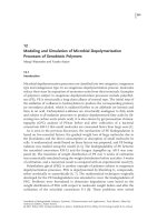
Figure 7.3. Introduction of a cutoff function.
Thus, the preceding analysis indicates that, for the three-dimensional case, an interaction
“cutoff” distance (d
c
) should be introduced (Figure 7.3),
||r
i
− r
j
|| = d
c
≤ d
(+)
, (7.14)
to avoid long-range (central-force) instabilities.
Remark. By introducing a cutoff distance, one can circumvent a loss-of-convexity
instability. However, introducing such acutoff can induce another type of instability. Specif-

ically, if the particles are in static equilibrium, or are not approaching one another, and if
the cutoff distance, d
c
, is much smaller than the static equilibrium separation distance, d
e
,
then the particles will not interact at all. Thus, we have the following two-sided bounds on
the cutoff for near-field forces to play a physically realistic role:

α
2
α
1

1
−β
1
+β
2
= d
(−)
≤ d
c
≤ d
(+)
=

β
2
α

2
β
1
α
1

1
−β
1
+β
2
. (7.15)
Clearly, since β
2
>β
1
, d
(−)
is a lower bound(dictatedbythe minimum interaction distance),
while d
(+)
is an upper bound (dictated by the (convexity-type) stability).
7.4 A simple model for thermochemical coupling
As indicated earlier, in certain applications, in addition to the near-field and contact effects
introduced thus far, thermal behavior is of interest. For example, applications arise in the
study of interstellar particulate dust flows in the presence of dilute hydrogen-rich gas. In
many cases, the source of heat generated during impact in such flows can be traced to the
reactivity of the particles. This affects the mechanics of impact, for example, due to thermal
softening. For instance, the presence of a reactive substance (gas) adsorbed onto the surface
of interplanetary dust can be a source of intense heat generation, through thermochemical

reactions activated by impact forces, which thermally softens the material, thus reducing the
coefficient of restitution, which in turn strongly affects the mechanical impact event itself
(Figure 7.4).
To illustrate how one can incorporate thermal effects, a somewhat ad hoc approach,
building on the relation in Equation (2.50), is to construct a thermally dependent coefficient
05 book
2007/5/15
page 59
✐
✐
✐
✐
✐
✐
✐
✐
7.4. A simple model for thermochemical coupling 59
REACTIVE FILM
TWO IMPACTING PARTICLES
ZOOM OF CONTACT AREA
Figure 7.4. Presence of dilute (smaller-scale) reactive gas particlesadsorbed onto
the surface of two impacting particles (Zohdi [217]).
of restitution as follows (multiplicative decomposition):
e
def
=

max

e

o

1 −
v
n
v
∗

,e
−

max

1 −
θ
θ
∗

, 0

, (7.16)
where θ
∗
can be considered as a thermal softening temperature. In order to determine the
thermal state of the particles, we shall decompose the heat generation and heat transfer
processes into two stages. Stage I describes the extremely short time interval when impact
occurs, δt  t, and accounts for the effects of chemical reactions, which are relevant in
certain applications, and energy release due to mechanical straining. Stage II accounts for
the postimpact behavior involving convective and radiative effects.
7.4.1 Stage I: An energy balance during impact

Throughout the analysis, we shall use extremely simple, basic, models. Consistent with
the particle-based philosophy, it is assumed that the temperature fields are uniform in the
particles.
30
We consider an energy balance, governing the interconversions of mechanical,
thermal, and chemical energy in a system, dictated by the first law of thermodynamics.
Accordingly, we require the time rate of change of the sum of the kinetic energy (K) and
the stored energy (S) to be equal to the sum of the work rate (power, P) and the net heat
supplied (H):
d
dt
(K + S) = P +H, (7.17)
where the stored energy comprises a thermal part,
S = mCθ, (7.18)
30
Thus, the gradient of the temperature within the particle is zero, i.e., ∇θ = 0. Thus, a Fourier-type law for
the heat flux will register a zero value, q =−K ·∇θ = 0.
05 book
2007/5/15
page 60
✐
✐
✐
✐
✐
✐
✐
✐
60 Chapter 7. Advanced particulate flow models
where C is the heat capacity per unit mass and, consistent with our assumptions that the

particles deform negligibly during impact, we assume that there is an insignificant amount
of mechanically stored energy. The kinetic energy is
K =
1
2
mv ·v. (7.19)
The mechanical power term is due to the forces acting on a particle, namely
P =
dW
dt
= 
tot
· v, (7.20)
and, because
dK
dt
= m
˙
v ·v, (7.21)
and we have a balance of momentum
m
˙
v ·v = 
tot
· v, (7.22)
we have
dK
dt
=
dW

dt
= P, (7.23)
leading to
dS
dt
= H. (7.24)
For example, in certain applications of interest, such as the ones mentioned, we consider that
the primary source of heat is due to chemical reactions, where the reactive layer generates
heat upon impact. The chemical reaction energy is defined as
δH
def
=

t+δt
t
H dt. (7.25)
Equation (7.24) can be rewritten for the temperature at time = t +δt as
θ(t + δt) = θ(t) +
δH
mC
. (7.26)
The energy released from the reactions is assumed to be proportional to the amount of the
gaseous substance available to be compressed in the contact area between the particles. A
typical ad hoc approximation in combustion processes is to write, for example, a linear
relation
δH ≈ κ min

|
I
n

|
I
∗
n
, 1

πb
2
, (7.27)
where I
n
is the normal impact force; κ is a reaction (saturation) constant, energy per unit
area; I
∗
n
is a normalization parameter; and b is the particle radius. For details, see Schmidt
[172], for example. For the grain sizes and material properties of interest, the term in
Equation (7.26),
δH
mC
, indicates that values of approximately κ ≈ 10
6
J/m
2
will generate
05 book
2007/5/15
page 61
✐
✐

✐
✐
✐
✐
✐
✐
7.4. A simple model for thermochemical coupling 61
significant amounts of heat.
31
Clearly, these equations are coupled to those of impact
through the coefficient of restitution and the velocity-dependent impulse. Additionally,
the postcollision velocities are computed from the momentum relations coupled to the
temperature. Later in the analysis, this equation is incorporated into an overall staggered
fixed-point iteration scheme, whereby the temperature is predicted for a given velocity field,
and then the velocities are recomputed with the new temperature field, etc. The process is
repeated until the fields change negligibly between successive iterations. The entire set of
equations are embedded within a larger overall set of equations later in the analysis and are
solved in a recursively staggered manner.
7.4.2 Stage II: Postcollision thermal behavior
After impact, it is assumed that a process of convection, for example, governed by Newton’s
law of cooling, and radiation, according to a simple Stefan–Boltzmann law, occurs. As be-
fore, it is assumed that the temperature fields are uniform within the particles, so conduction
within the particles is negligible. We remark that the validity of using a lumped thermal
model, i.e., ignoring temperature gradients and assuming a uniform temperature within a
particle, is dictated by the magnitude of the Biot number. A small Biot number indicates
that such an approximation is reasonable. The Biot number for spheres scales with the ratio
of the particle volume (V ) to the particle surface area (a
s
),
V

a
s
=
b
3
, which indicates that a
uniform temperature distribution is appropriate, since the particles, by definition, are small.
We also assume that the dynamics of the (dilute) gas does not affect the motion of the (much
heavier) particles. The gas only supplies a reactive thin film on the particles’ surfaces. The
first law reads
d(K +U)
dt
= m
˙
v ·v + mC
˙
θ = 
tot
· v

 
mechanical power
− h
c
a
s
(θ − θ
o
)


 
convective heating
−Ba
s
(θ
4
− θ
4
s
)

 
far-field radiation
, (7.28)
where θ
o
is the temperature of the ambient gas; θ
s
is the temperature of the far-field surface
(for example, a container surrounding the flow) with which radiative exchange is made;
B = 5.67 × 10
−8
W
m
2
−K
is the Stefan–Boltzmann constant; 0 ≤  ≤ 1 is the emissivity,
which indicates how efficiently the surface radiates energy compared to a black-body (an
ideal emitter); 0 ≤ h
c

is the heating due to convection (Newton’s law of cooling) into
the dilute gas; and a
s
is the surface area of a particle. It is assumed that the radiation
exchange between the particles (emission exchange between particles) is negligible.
32
For
the applications considered here, typically, h
c
is quite small and plays a small role in the
heat transfer processes.
33
From a balance of momentum, we have m
˙
v · v = 
tot
· v, and
Equation (7.28) becomes
mC
˙
θ =−h
c
a
s
(θ − θ
o
) − Ba
s
(θ
4

− θ
4
s
).
(7.29)
31
By construction, this model has increased heat production, via δH, for increasing κ.
32
Various arguments for such an assumption can be found in the classical text of Bohren and Huffman [33].
33
The Reynolds number, which measures the ratio of the inertial forces to viscous forces in the surrounding gas
and dictates the magnitude of these parameters, is extremely small in the regimes considered.
05 book
2007/5/15
page 62
✐
✐
✐
✐
✐
✐
✐
✐
62 Chapter 7. Advanced particulate flow models
Therefore, after temporal integration with the previously used finite difference time step of
t  δt, we have
34
θ(t + t) =
mC
mC + h

c
a
s
t
¯
θ(t) −
tBa
s

mC + h
c
a
s
t

θ
4
(t +t) −θ
4
s

+
h
c
a
s
tθ
o
mC + h
c

a
s
t
,
(7.30)
where
¯
θ(t)
def
= θ(t+δt) is computed from Equation (7.26). This implicit nonlinear equation
for θ(t + t), for each particle, is solved simultaneously with the equations for the dy-
namics of the particles by employing a multifield staggering scheme, which we shall discuss
momentarily.
Remark. Convection heat transfer comprises two primary mechanisms, one due to
primarily random molecular motion (diffusion) and the other due to bulk motion of a fluid,
in our case a gas, surrounding the particles. As we have indicated, in the applications of
interest, the gas is dilute and the Reynolds number is small, so convection plays a very
small role in the heat transfer process for dry particulate flows in the presence of a dilute
gas. The nondilute surrounding fluid case will be considered in Chapter 8. Also, we recall
that a black-body is an ideal radiating surface with the following properties:
• A black-body absorbs all incident radiation, regardless of wavelength and direction.
• For a prescribed temperature and wavelength, no surface can emit more energy than
a black-body.
• Although the radiation emitted by a black-body is a function of wavelength and
temperature, it is independent of direction.
Since a black-body is a perfect emitter, it serves as a standard against which the radia-
tive properties of actual surfaces may be compared. The Stefan–Boltzmann law, which is
computed by integrating the Planck representation of the emissive power distribution of a
black-body over all wavelengths,
35

allows the calculation of the amount of radiation emitted
in all directions and over all wavelengths simply from the knowledge of the temperature of
the black-body. We note that Equation (7.30) is of the form
θ(t + t) = G(θ (t + t)) + R, (7.31)
where R = R(θ(t +t)) and G’s behavior is controlled by
tBa
s

mC + h
c
a
s
t
, (7.32)
which is quite small. Thus, a fixed-point iterative scheme such as
θ
K
(t +t) = G(θ
K−1
(t +t)) +R (7.33)
would converge rapidly.
34
For this stage, since δt  t, we assign θ(t) = θ(t + δt) = θ(t) +
δH
mC
and replace θ(t) with it in Equation
(7.30).
35
Radiation is idealized as requiring no medium to transmit energy.
05 book

2007/5/15
page 63
✐
✐
✐
✐
✐
✐
✐
✐
7.5. Staggering schemes 63
7.5 Staggering schemes
Broadly speaking, staggering schemes proceed by solving each field equation individually,
allowing only the primary field variable to be active. After the solution of each field
equation, the primary field variable is updated, and the next field equation is addressed in
a similar manner. Such approaches have a long history in the computational mechanics
community. For example, see Park and Felippa [161], Zienkiewicz [206], Schrefler [173],
Lewis et al. [133], Doltsinis [52], [53], Piperno [162], Lewis and Schrefler [132], Armero
and Simo [7]–[9], Armero [10], Le Tallec and Mouro [131], Zohdi [208], [209], and the
extensive works of Farhat and coworkers (Piperno et al. [163], Farhat et al. [65], Lesoinne
and Farhat [130], Farhat and Lesoinne [66], Piperno and Farhat [163], andFarhat et al.[67]).
Generally speaking, if a recursive staggering process is not employed (an explicit scheme),
the staggering error can accumulate rapidly. However, an overkill approach involving
very small time steps, smaller than needed to control the discretization error, simply to
suppress a nonrecursive staggering process error, is computationally inefficient. Therefore,
the objective ofthenextsectionistodevelopa strategy to adaptively adjust, in fact maximize,
the choice of the time step size to control the staggering error, while simultaneously staying
below the critical time step size needed to control the discretization error. An important
related issue is to simultaneously minimize the computational effort involved. The number
of times the multifield system is solved, as opposed to time steps, is taken as the measure

of computational effort, since within a time step, many multifield system re-solves can take
place. We now develop a staggering scheme by following an approach found in Zohdi
[208]–[210].
7.5.1 A general iterative framework
We consider an abstract setting, whereby one solves for the particle positions, assuming the
thermal fields fixed,
A
1
(r
L+1,K
,θ
L+1,K−1
) = F
1
(r
L+1,K−1
,θ
L+1,K−1
), (7.34)
and then one solves for the thermal fields, assuming the particle positions fixed,
A
2
(r
L+1,K
,θ
L+1,K
) = F
2
(r
L+1,K

,θ
L+1,K−1
), (7.35)
where only the underlined variable is “active,” L indicates the time step, and K indicates
the iteration counter. Within the staggering scheme, implicit time-stepping methods, with
time step size adaptivity, will be used throughout the upcoming analysis.
Continuing where Equation (3.28) left off, we define the normalized errors within
each time step, for the two fields, as

rK
def
=
||r
L+1,K
− r
L+1,K−1
||
||r
L+1,K
− r
L
||
and 
θK
def
=
||θ
L+1,K
− θ
L+1,K−1

||
||θ
L+1,K
− θ
L
||
.
(7.36)
We define the maximum “violation ratio,” i.e., the larger of the ratios of each field variable’s
error to its corresponding tolerance, by Z
K
def
= max(z
rK
,z
θK
), where
z
rK
def
=

rK
TOL
r
and z
θK
def
=


θK
TOL
θ
,
(7.37)
05 book
2007/5/15
page 64
✐
✐
✐
✐
✐
✐
✐
✐
64 Chapter 7. Advanced particulate flow models
with the minimum scaling factor defined as 
K
def
= min(φ
rK
,φ
θK
), where
φ
rK
def
=




TOL
r

r0

1
pK
d


rK

r0

1
pK


,φ
θK
def
=



TOL
θ


θ0

1
pK
d


θK

θ0

1
pK


. (7.38)
SeeAlgorithm 7.1. The overall goal is to deliver solutions where the staggering (incomplete
coupling) error is controlled and the temporal discretization accuracy dictates the upper
limits on the time step size (t
lim
).
Remark. As in the single-field multiple-particle discussion earlier, an alternative
approach is to attempt to solve the entire multifield system simultaneously (monolithically).
This would involve the use of a Newton-type scheme, which can also be considered as a
type of fixed-point iteration. Newton’s method is covered as a special case of this general
analysis. To see this, let
w = (r,θ), (7.39)
and consider the residual defined by

def

= A(w) − F . (7.40)
Linearization leads to
(w
K
) = (w
K−1
) +∇
w
|
w
K−1
(w
K
− w
K−1
) + O(||w||
2
), (7.41)
and thus the Newton updating scheme can be developed by enforcing
(w
K
) ≈ 0, (7.42)
leading to
w
K
= w
K−1
− (A
TAN ,K−1
)

−1
(w
K−1
), (7.43)
where
A
TAN ,K
=
(
∇
w
A(w)
)
|
w
K
=
(
∇
w
(w)
)
|
w
K
(7.44)
is the tangent. Therefore, in the fixed-point form, one has the operator
G(w) = w − (A
TAN
)

−1
(w). (7.45)
One immediately sees a fundamental difficulty due to the possibility of a zero or near-zero
tangent when employing a Newton’s method on a nonconvex system, whichcan lose positive
definiteness and which in turn will lead to an indefinite system of algebraic equations.
36
Therefore, while Newton’s method usually converges at a faster rate than a direct fixed-
point iteration, quadratically as opposed to superlinearly, its convergence criteria are less
robust than the presented fixed-point algorithm, due to its dependence on the gradients of
the solution. Furthermore, for the problems considered, the solutions are nonsmooth and
nonconvex, primarily due to the impact events, and thus we opted for the more robust
“gradientless” staggering scheme.
36
Furthermore, the tangent may not exist in some (nonsmooth) cases.
05 book
2007/5/15
page 65
✐
✐
✐
✐
✐
✐
✐
✐
7.5. Staggering schemes 65
(1) GLOBAL FIXED-POINT ITERATION (SET i = 1 AND K = 0):
(2) IF i>N
p
, THEN GO TO (4);

(3) IF i ≤ N
p
, THEN (FOR PARTICLE i)
(a) COMPUTE POSITION: r
L+1,K
i
≈
t
2
m


tot
(r
L+1,K−1
)

+ r
L
i
+ t
˙
r
L
i
;
(b) COMPUTE TEMPERATURE (FOR PARTICLE i):
θ
L+1,K
i

= θ
L
i
+
δH
L+1,K−1
mC
;
θ
L+1,K
i
=
mC
mC + h
c
a
s
t
θ
L+1,K−1
i
−
tBa
s

mC + h
c
a
s
t


(θ
L+1,K−1
i
)
4
− θ
4
s

+
h
c
a
s
tθ
o
mC + h
c
a
s
t
;
(c) GO TO (2) AND NEXT PARTICLE (i = i + 1);
(4) ERROR MEASURES (normalized):
(a) 
rK
def
=


N
p
i=1
||r
L+1,K
i
− r
L+1,K−1
i
||

N
p
i=1
||r
L+1,K
i
− r
L
i
||
,
θK
def
=

N
p
i=1
||θ

L+1,K
i
− θ
L+1,K−1
i
||

N
p
i=1
||θ
L+1,K
i
− θ
L
i
||
;
(b) Z
K
def
= max(z
rK
,z
θK
) where z
rK
def
=


rK
TOL
r
,z
θK
def
=

θK
TOL
θ
;
(c) 
K
def
= min(φ
rK
,φ
θK
) where φ
rK
def
=




TOL
r


r0

1
pK
d


rK

r0

1
pK



,
φ
θK
def
=




TOL
θ

θ0


1
pK
d


θK

θ0

1
pK



;
(5) IF TOLERANCE MET (Z
K
≤ 1) AND K<K
d
, THEN
(a) INCREMENT TIME: t = t + t;
(b) CONSTRUCT NEW TIME STEP: t = 
K
t;
(c) SELECT MINIMUM: t = min(t
lim
,t)AND GO TO (1);
(6) IF TOLERANCE NOT MET (Z
K
> 1) AND K = K

d
, THEN:
(a) CONSTRUCT NEW TIME STEP: t = 
K
t;
(b) RESTART AT TIME = t AND GO TO (1).
Algorithm 7.1
05 book
2007/5/15
page 66
✐
✐
✐
✐
✐
✐
✐
✐
66 Chapter 7. Advanced particulate flow models
7.5.2 Semi-analytical examples
For the class of coupled systems considered in this work, the coupled operator’s spectral
radius is directly dependent on the timestepdiscretizationt. Weconsiderasimpleexample
that illustrates the essential concepts. Consider the coupling of two first-order equations
and one second-order equation
a ˙w
1
+ w
2
= 0,
b ˙w

2
+ w
3
= 0,
c ¨w
3
+ w
1
= 0.
(7.46)
When this is discretized in time, for example, with a backward Euler scheme, we obtain
˙w
1
L+1
=
w
L+1
1
− w
L
1
t
,
˙w
2
L+1
=
w
L+1
2

− w
L
2
t
,
¨w
3
L+1
=
w
L+1
3
− 2w
L
3
+ w
L−1
3
(t)
2
,
(7.47)
which leads to the following coupled system:



1
t
a
0

01
t
b
(t)
2
c
01








w
L+1
1
w
L+1
2
w
L+1
3





=






w
L
1
w
L
2
2w
L
3
− w
L−1
3





. (7.48)
For a recursive staggering scheme of Jacobi type, where the updates are made only after
one complete iteration, considered here only for algebraic simplicity, we have
37



100

010
001








w
L+1,K
1
w
L+1,K
2
w
L+1,K
3





=






w
L
1
w
L
2
2w
L
3
− w
L−1
3





−







t
a
w
L+1,K−1
1

t
b
w
L+1,K−1
2
(t)
2
c
w
L+1,K−1
3







. (7.49)
Rewriting this in terms of the standard fixed-point form, G(w
L+1,K−1
) + R = w
L+1,K
,
yields



0
t

a
0
00
t
b
(t)
2
c
00



  
G





w
L+1,K−1
1
w
L+1,K−1
2
w
L+1,K−1
3







 
w
L+1,K−1
+





w
L
1
w
L
2
2w
L
3
− w
L−1
3







 
R
=





w
L+1,K
1
w
L+1,K
2
w
L+1,K
3






 
w
L+1,K
. (7.50)
37
A Gauss–Seidel approach would involve using the most current iterate. Typically, under very general con-

ditions, if the Jacobi method converges, the Gauss–Seidel method converges at a faster rate, while if the Jacobi
method diverges, the Gauss–Seidel method diverges at a faster rate. For example, see Ames [5] for details. The
Jacobi method is easier to address theoretically, so it is used for proof of convergence, and the Gauss–Seidel
method is used at the implementation level.
05 book
2007/5/15
page 67
✐
✐
✐
✐
✐
✐
✐
✐
7.5. Staggering schemes 67
The eigenvalues of G are given by λ
3
=
(t)
4
abc
and, hence, for convergence we must have
|max λ|=




(t)
4

abc




1
3
< 1. (7.51)
We see that the spectral radius of the staggering operator grows quasi-linearly with the
time step size, specifically superlinearly as (t)
4
3
. Following Zohdi [208], a somewhat
less algebraically complicated example illustrates a further characteristic of such solution
processes. Consider the following example of reduced dimensionality, namely, a coupled
first-order system
a ˙w
1
+ w
2
= 0,
b ˙w
2
+ w
1
= 0.
(7.52)
When discretized in time with a backward Euler scheme and repeating the preceding pro-
cedure, we obtain the G-form


0
t
a
t
b
0


 
G

w
L+1,K−1
1
w
L+1,K−1
2


 
w
L+1,K−1
+

w
L
1
w
L
2



 
R
=

w
L+1,K
1
w
L+1,K
2


 
w
L+1,K
. (7.53)
The eigenvalues of G are
λ
1,2
=±

(t)
2
ab
. (7.54)
We see that the convergence of the staggering scheme is directly related (linearly in this
case) to the size of the time step. The solution to the example is
w

L+1
1
=
abw
L
1
+ btw
L
2
ab −(t)
2
= w
L
1
−
w
L
2
a
t

 
first staggered iteration
+
w
L
1
ab
(t)
2

  
second staggered iteration
+···
(7.55)
and
w
L+1
2
=
abw
L
2
+ atw
L
1
ab −(t)
2
= w
L
2
−
w
L
1
b
t
  
first staggered iteration
+
w

L
2
ab
(t)
2
  
second staggered iteration
+···.
(7.56)
As pointed out in Zohdi [208], the time step induced restriction for convergence matches
the radius of analyticity of a Taylor series expansion of the solution around time t, which
converges in a ball of radius from the point of expansion to the nearest singularity in
Equations (7.55) and (7.56). In other words, the limiting step size is given by setting the
denominator to zero,
ab −(t)
2
= 0, (7.57)
which is in agreement with the condition derived from the analysis of the eigenvalues of G.
05 book
2007/5/15
page 68
✐
✐
✐
✐
✐
✐
✐
✐
68 Chapter 7. Advanced particulate flow models

Remark. Clearly, 1 ≤ p ≤ 2 for a collection of first- and second-order equations.
However, sincewe choose the individual field with themaximum error for timestep adaptiv-
ity, we need to specifically use the corresponding convergence exponent (p) for the selected
field’s temporal discretization. If the equations of dynamic equilibrium of the particles are
chosen, then p = 2, while if the equations of thermodynamic equilibrium of the particles
are chosen, then p = 1. This issue is discussed further later in the analysis.
7.5.3 Numerical examples involving particulate flows
In order to simulate a particulate flow, we considered a group of N
p
randomly positioned
particles, of equal size, in a (starting) cubical domain of dimensions D × D × D, with
D normalized to unity. The particle size and volume fraction were determined by a par-
ticle/sample size ratio, which was defined via a subvolume size V
def
=
D×D×D
N
p
, where
N
p
was the number of particles in the entire cube. The ratio between the radius (b) and the
subvolume was denoted by L
def
=
b
V
1
3
. The volume fraction occupied by the particles was

v
f
def
=
4πL
3
3
. Thus, thetotal volume occupied by the particles, denoted by ν, could be written
as ν = v
f
N
p
V , and the total mass could be written as M =

N
p
i=1
m
i
= ρν, while that of
an individual particle, assuming that all are the same size, was m
i
=
ρν
N
p
= ρ
4
3
πb

3
i
. In order
to visualize the flow clearly, we used N
p
= 100 particles. The length scale of the particles
was L = 0.25, which resulted in a corresponding volume fraction of v
f
=
4πL
3
3
= 0.0655
and particulate radii of b = 0.0539. A mass density of the particles = 2000 kg/m
3
was
used. The ambient temperature was selected to be θ
o
= θ
s
= 300
◦
K. The heat capacity of
the particles was C = 10
3
J/kg
◦
K, with emissivity of  = 10
−2
. The critical temperature

parameter in the coefficient of restitution relation was θ
∗
= 3000
◦
K. The reaction constant
was varied in the range 10
6
J/m
2
≤ κ ≤ 10
7
J/m
2
, with I
∗
= 10
3
N. The coefficient of
convective heat transfer (h
c
) was set to zero. We introduced the following near-field param-
eters per unit mass
2
: α
1ij
= α
1
m
i
m

j
, α
2ij
= α
2
m
i
m
j
, and α
aij
= α
a
m
i
m
j
. This allowed
us to scale the strength of the interaction forces according to the mass of the particles.
38
The initial mean velocity field, componentwise, was (1.0, 0.1, 0.1) m/s with initial random
perturbations around the mean velocity of (±1.0, ±0.1, ±0.1) m/s, and a critical threshold
velocity of v
∗
= 10 m/s in Equation (7.16). The simulation duration was set to 5 s, with an
upper bound on the time step size of t
lim
= 10
−2
s and a starting time step size of 10

−3
s.
The tolerances of both fields (TOL
r
and TOL
θ
) for the fixed-point iterations were set to 10
−6
and the upper limit on the number of fixed-point iterations was set to K
d
= 10
2
.
Two main types of computational tests were conducted:
1. varying κ, for a given field strength,
α
1
= 0.5 and α
2
= 0.25, with a clustering
augmentation of
α
a
= 1.75 (forcing a small gap characterized by d
a
= 1.03(2b)),
β
a
= 1, δ
a

= 1.65(2b), and
2. varying κ, for a given field strength,
α
1
= 0.5 and α
2
= 0.25, without a clustering
augmentation.
38
Although we did not consider particles of different sizes in this example, this decomposition allows us to
easily take this into account. Also, we enforced the near-field stability condition by setting (β
1
,β
2
) = (1, 2).
05 book
2007/5/15
page 69
✐
✐
✐
✐
✐
✐
✐
✐
7.5. Staggering schemes 69
XY
Z
XY

Z
XY
Z
XY
Z
Figure 7.5. Top to bottom and left to right, the dynamics of the particulate flow
with clustering forces: An initially fine cloud of particles that clusters to form structures
within the flow. Blue indicates a temperature of approximately 300
◦
K, while red indicates
a temperature of approximately 400
◦
K (Zohdi [217]).
For each different parameter selection, the initial conditions, i.e., random positions,
velocities, temperatures, etc., were the same. We remark that parameter studies on the near-
field strength, in isolation (without thermochemical coupling), havebeenconductedinZohdi
[209]. The field strength chosen was strong enough to induce vibratory motion and hence
nonmonotone kinetic energy. Frames of the flows for cases 1 and 2, for (typical) values of
κ = 2 ×10
6
J/m
2
, are shown in Figures 7.5 and 7.6. The plots in Figures 7.7–7.10 indicate
the overall energetic and thermal behavior. Typically, the simulations took approximately
between 1 min and 2 min on a standard (Dell, 2.33 GHz) laptop.
39
For the parameter ranges
used in the presented simulations, the degree of adaptivity needed strongly depended on the
presence of the clustering forces, and to a somewhat lesser degree on the thermochemical
parameters. For example, for the 5-s simulation, if the time steps stayed at the starting value

39
The computationtime scaleswere, approximately, noworse thanthe number of particles squared. For example,
a thousand particles took approximately 10 min.
05 book
2007/5/15
page 70
✐
✐
✐
✐
✐
✐
✐
✐
70 Chapter 7. Advanced particulate flow models
XY
Z
XY
Z
XY
Z
XY
Z
Figure 7.6. Top to bottom and left to right, the dynamics of the particulate flow
without clustering forces. Blue indicates a temperature of approximately 300
◦
K, while red
indicates a temperature of approximately 400
◦
K (Zohdi [217]).

(t = 10
−3
s), then 5000 timestepswouldbe needed if therehadbeenno time step adaptivity
(time step enlargement). Conversely, if the time steps were found to be unnecessarily small
(an overkill) at the starting value (t = 10
−3
s), and, consequently, unrefined to the upper
bound (t
lim
= 10
−2
s), then approximately500 timesteps wouldbe needed. Tables 7.1 and
7.2 indicate that, for the parameter ranges tested, when clustering forces were not present,
the time steps did not need to be refined or unrefined. However, when clustering forces were
present, the time steps could be unrefined for the given tolerances, requiring more internal
fixed-point iterations. This was primarily because cluster structures formed, leading to
fewer collisions between the larger objects, which did not require such small time steps
(Figure 7.11). For the simulations with clustering forces, there was an expected thermal
sensitivity. As the reaction constant κ became stronger, the number of fixed-point iterations
required to achieve convergence increased. These results highlight an essential point of the
adaptive time-stepping process, which is to allow the system to adjust to the physics of the
problem. Some furtherremarks elaborating on this issuecan be found in Zohdi [208]–[210].
05 book
2007/5/15
page 71
✐
✐
✐
✐
✐

✐
✐
✐
7.5. Staggering schemes 71
0.4
0.45
0.5
0.55
0.6
0.65
0.7
0.75
0 0.5 1 1.5 2 2.5 3 3.5 4 4.5 5
ENERGY (N-m)
TIME
TOTAL KINETIC ENERGY
0.4
0.45
0.5
0.55
0.6
0.65
0.7
0.75
0 0.5 1 1.5 2 2.5 3 3.5 4 4.5 5
ENERGY (N-m)
TIME
TOTAL KINETIC ENERGY
0.4
0.45

0.5
0.55
0.6
0.65
0.7
0.75
0 0.5 1 1.5 2 2.5 3 3.5 4 4.5 5
ENERGY (N-m)
TIME
TOTAL KINETIC ENERGY
0.4
0.45
0.5
0.55
0.6
0.65
0.7
0.75
0 0.5 1 1.5 2 2.5 3 3.5 4 4.5 5
ENERGY (N-m)
TIME
TOTAL KINETIC ENERGY
Figure 7.7. Top to bottom and left to right, with clustering forces: the total kinetic
energy in the system per unit mass with e
o
= 0.5, µ
s
= 0.2, µ
d
= 0.1, α

1
= 0.5, and
α
2
= 0.25: (1) κ = 10
6
J/m
2
, (2) κ = 2 × 10
6
J/m
2
, (3) κ = 4 × 10
6
J/m
2
, and (4)
κ = 8 × 10
6
J/m
2
(Zohdi [217]).
Qualitatively speaking, one should expect that, when aclustering field becomes active
between two approaching particles, then kinetic energy is lost because of the disappearance
of normal relative velocities between them. Conversely, kinetic energy is gained ifthe parti-
cles become dislodged, because the clustering field becomes inactive and the repulsive field
suddenly dominates the remaining attractive forces, thus pushing the previously clustered
particles away from one another. When the clustering binding field becomes active, the
coefficient of restitution will play virtually no role, because the strength of the attractive
force dominates everything. Thus, because the thermal field affects the particle dynamics

through the coefficient of restitution, when clustering dominates, the particle dynamics will
be only marginally affected by varying κ (Figure 7.7). However, the temperature of the
particles in the presence of clustering will rise substantially, due to the large compressive
forces between the contacting particles, which activate the chemical reactions. Also, we
remark that the group dynamics, for different κ without clustering forces, deviate much
more from one another than the cases when clustering is present (Figure 7.8). Typically,
when two particles have clustered, since the binding field was strong, the particles rarely
become dislodged. This issue has been been investigated in depth in Zohdi [225].
05 book
2007/5/15
page 72
✐
✐
✐
✐
✐
✐
✐
✐
72 Chapter 7. Advanced particulate flow models
0.6
0.61
0.62
0.63
0.64
0.65
0.66
0.67
0.68
0.69

0.7
0 0.5 1 1.5 2 2.5 3 3.5 4 4.5 5
ENERGY (N-m)
TIME
TOTAL KINETIC ENERGY
0.6
0.61
0.62
0.63
0.64
0.65
0.66
0.67
0.68
0.69
0.7
0 0.5 1 1.5 2 2.5 3 3.5 4 4.5 5
ENERGY (N-m)
TIME
TOTAL KINETIC ENERGY
0.6
0.61
0.62
0.63
0.64
0.65
0.66
0.67
0.68
0.69

0.7
0 0.5 1 1.5 2 2.5 3 3.5 4 4.5 5
ENERGY (N-m)
TIME
TOTAL KINETIC ENERGY
0.6
0.61
0.62
0.63
0.64
0.65
0.66
0.67
0.68
0.69
0.7
0 0.5 1 1.5 2 2.5 3 3.5 4 4.5 5
ENERGY (N-m)
TIME
TOTAL KINETIC ENERGY
Figure 7.8. Top to bottom and left to right, without clustering forces: the total
kinetic energy in the system per unit mass with e
o
= 0.5, µ
s
= 0.2, µ
d
= 0.1, α
1
= 0.5,

and
α
2
= 0.25: (1) κ = 10
6
J/m
2
, (2) κ = 2 × 10
6
J/m
2
, (3) κ = 4 × 10
6
J/m
2
, and (4)
κ = 8 × 10
6
J/m
2
(Zohdi [217]).
Remark. The interaction of clouds of granular gases with large (essentially im-
movable) obstacles arises in a variety of applications. It follows that associated impact
phenomena are important. Accordingly, consider a stationary, massive obstacle (M  m)
of radius b
ob
. For this example, we assume that the obstacle has no near-field interaction
with the particles, other than contact, which is governed by the classical expression for the
ratio of the relative velocities before and after impact:
e

def
=
v
obn
(t +δt) − v
in
(t +δt)
v
in
(t) − v
obn
(t)
,
(7.58)
where v
obn
remains the same before and after impact. In Figure 7.13, the impact of a cloud
against an obstacle is shown.
40
Let us focus on a particle impacting a massive obstacle
M  m (Figure 7.12). A balance of momentum reads for the particle as
mv(t) −
¯
Iδt ±|
¯
F |δt = mv(t + δt). (7.59)
40
All other parameters are the same as in the previous simulations.
05 book
2007/5/15

page 73
✐
✐
✐
✐
✐
✐
✐
✐
7.5. Staggering schemes 73
298
300
302
304
306
308
310
312
314
316
318
320
0 0.5 1 1.5 2 2.5 3 3.5 4 4.5 5
TEMPERATURE
TIME
TEMPERATURE
300
305
310
315

320
325
330
335
340
0 0.5 1 1.5 2 2.5 3 3.5 4 4.5 5
TEMPERATURE
TIME
TEMPERATURE
300
400
500
600
700
800
900
1000
0 0.5 1 1.5 2 2.5 3 3.5 4 4.5 5
TEMPERATURE
TIME
TEMPERATURE
200
400
600
800
1000
1200
1400
1600
1800

0 0.5 1 1.5 2 2.5 3 3.5 4 4.5 5
TEMPERATURE
TIME
TEMPERATURE
Figure 7.9. Top to bottom and left to right, with clustering forces: the average
particle temperature with e
o
= 0.5, µ
s
= 0.2, µ
d
= 0.1, α
1
= 0.5, and α
2
= 0.25: (1)
κ = 10
6
J/m
2
, (2) κ = 2 × 10
6
J/m
2
, (3) κ = 4 × 10
6
J/m
2
, and (4) κ = 8 × 10
6

J/m
2
(Zohdi [217]).
The coefficient of restitution reads as
e
def
=
−v
in
(t +δt)
v
in
(t)
,
(7.60)
so
¯
I =−
m(v(t +δt) −v(t)
δt
±|
¯
F |=−
mv(t)(1 +e)
δt
±|
¯
F |, (7.61)
where ±|
¯

F | becomes |
¯
F | if attractive and −|
¯
F | if repulsive. Thus, we should expect that
the impact of the aggregate will generally be lower if the interstitial forces are attractive at
impact and that the impact of the aggregate will generally be higher if the interstitial forces
are repulsive at impact. In order to illustrate this point, we consider two cases:
1. a given interaction field strength,
α
1
= 0.5 and α
2
= 0.25,
2. no interaction field strength.
The results for a cloud of particles are shown in Figures 7.14 and 7.15.
05 book
2007/5/15
page 74
✐
✐
✐
✐
✐
✐
✐
✐
74 Chapter 7. Advanced particulate flow models
300
301

302
303
304
305
306
307
0 0.5 1 1.5 2 2.5 3 3.5 4 4.5 5
TEMPERATURE
TIME
TEMPERATURE
298
300
302
304
306
308
310
312
0 0.5 1 1.5 2 2.5 3 3.5 4 4.5 5
TEMPERATURE
TIME
TEMPERATURE
300
305
310
315
320
325
330
0 0.5 1 1.5 2 2.5 3 3.5 4 4.5 5

TEMPERATURE
TIME
TEMPERATURE
300
310
320
330
340
350
360
370
380
390
400
0 0.5 1 1.5 2 2.5 3 3.5 4 4.5 5
TEMPERATURE
TIME
TEMPERATURE
Figure 7.10. Top to bottom and left to right, without clustering forces: the average
particle temperature with e
o
= 0.5, µ
s
= 0.2, µ
d
= 0.1, α
1
= 0.5, and α
2
= 0.25: (1)

κ = 10
6
J/m
2
, (2) κ = 2 × 10
6
J/m
2
, (3) κ = 4 × 10
6
J/m
2
, and (4) κ = 8 × 10
6
J/m
2
(Zohdi [217]).
Table 7.1. The number of time steps and fixed-point iterations, with clustering
forces: the average particle temperature with e
o
= 0.5, µ
s
= 0.2, µ
d
= 0.1, α
1
= 0.5, and
α
2
= 0.25.

κ(J ×10
6
/m
2
) Time Steps Fixed-Point Iterations
1 586 1730
2 588 2076
4
598 4809
8 596 5584
Remark. Clearly, during flow processes, there is a possibility that the agglomer-
ated clouds may impact one another and fragment as a result. In Figure 7.16, cloud
collisions for slow approaching impact are shown, and in Figure 7.17 fast cloud im-
pact is given.
41
A gallery of cloud interaction simulations can be found at http://
www.siam.org/books/cs04.
41
All other parameters are the same as in the previous simulations. In the case of slow impact, the clouds
combine to form a larger cloud, and when the impact is fast, they disperse.
05 book
2007/5/15
page 75
✐
✐
✐
✐
✐
✐
✐

✐
7.5. Staggering schemes 75
Table 7.2. The number of time steps and fixed-point iterations, without clustering
forces: the average particle temperature with e
o
= 0.5, µ
s
= 0.2, µ
d
= 0.1, α
1
= 0.5, and
α
2
= 0.25.
κ(J ×10
6
/m
2
)
Time Steps Fixed-Point Iterations
1 5000 5025
2 5000 5024
4
5000 5029
8 5000 5024
XY
Z
Figure 7.11. A zoom on the structures that form with clustering. Blue indicates a
temperature of approximately 300

◦
K, while red indicates a temperature of approximately
400
◦
K (Zohdi [217]).
F
(CHARGED) (UNCHARGED)
Figure 7.12. Cases with and without charging.
05 book
2007/5/15
page 76
✐
✐
✐
✐
✐
✐
✐
✐
76 Chapter 7. Advanced particulate flow models
X
Y
Z
X
Y
Z
X
Y
Z
X

Y
Z
Figure 7.13. Top to bottom and leftto right, a charged cloud against animmovable
obstacle.