An Introduction to Modeling and Simulation of Particulate Flows Part 6 pps

05 book
2007/5/15
page 77
✐
✐
✐
✐
✐
✐
✐
✐
7.5. Staggering schemes 77
0
5e+07
1e+08
1.5e+08
2e+08
2.5e+08
3e+08
3.5e+08
0 0.1 0.2 0.3 0.4 0.5 0.6 0.7 0.8 0.9 1
MAXIMUM FORCE (N)
TIME
NORMAL FORCE
TANGENTIAL FORCE
0
5e+07
1e+08
1.5e+08
2e+08
2.5e+08

3e+08
3.5e+08
0 0.1 0.2 0.3 0.4 0.5 0.6 0.7 0.8 0.9 1
MAXIMUM FORCE (N)
TIME
NORMAL FORCE
TANGENTIAL FORCE
Figure 7.14. The maximum force (and corresponding friction force) versus time
imparted on the immovable obstacle surface, max(
I). The top graph is with charging and
the bottom is without charging. Notice that the maximum “signature” force is less with
charging.
05 book
2007/5/15
page 78
✐
✐
✐
✐
✐
✐
✐
✐
78 Chapter 7. Advanced particulate flow models
-5e+08
-4e+08
-3e+08
-2e+08
-1e+08
0

1e+08
2e+08
3e+08
4e+08
0 0.1 0.2 0.3 0.4 0.5 0.6 0.7 0.8 0.9 1
TOTAL FORCE (N)
TIME
TOTAL X NORMAL FORCE
TOTAL Y NORMAL FORCE
TOTAL Z NORMAL FORCE
TOTAL X TANGENTIAL FORCE
TOTAL Y TANGENTIAL FORCE
TOTAL Z TANGENTIAL FORCE
-6e+08
-4e+08
-2e+08
0
2e+08
4e+08
6e+08
8e+08
0 0.1 0.2 0.3 0.4 0.5 0.6 0.7 0.8 0.9 1
TOTAL FORCE (N)
TIME
TOTAL X NORMAL FORCE
TOTAL Y NORMAL FORCE
TOTAL Z NORMAL FORCE
TOTAL X TANGENTIAL FORCE
TOTAL Y TANGENTIAL FORCE
TOTAL Z TANGENTIAL FORCE

Figure 7.15. The total force (and corresponding friction force) versus time im-
parted on the immovable obstacle surface, max(
I). The top graph is with charging and the
bottom is without charging. Notice that the total “signature” force is less with charging.
05 book
2007/5/15
page 79
✐
✐
✐
✐
✐
✐
✐
✐
7.5. Staggering schemes 79
X Y
Z
X Y
Z
X Y
Z
X Y
Z
Figure 7.16. Top to bottom and left to right, slow impact of charged clouds. The
clouds combine into a larger cloud.
05 book
2007/5/15
page 80
✐

✐
✐
✐
✐
✐
✐
✐
80 Chapter 7. Advanced particulate flow models
X Y
Z
X Y
Z
X Y
Z
X Y
Z
Figure 7.17. Top to bottom and left to right, fast impact of charged clouds. The
clouds disperse.
05 book
2007/5/15
page 81
✐
✐
✐
✐
✐
✐
✐
✐
Chapter 8

Coupled particle/fluid
interaction
Until this point, we have ignored the presence of a fluid medium surrounding the particles.
We now focus on the modeling and simulation of the dynamics of particles, coupled with a
surrounding fluid, while bringing in several of the effects discussed earlier in the form of a
model problem. Obviously, the number of research areas involving particles in a fluid un-
dergoing various multifield processesis immense, andit would be futileto attempt to catalog
all ofthe various applications. However, a common characteristic of such systems is that the
various physical fields (thermal, mechanical,chemical, electrical, etc.) are strongly coupled.
This chapter develops a flexible and robust solution strategy to resolve coupled sys-
tems comprising large groups of flowing particles embedded within a fluid. A problem
modeling groups of particles, which may undergo inelastic collisions in the presence of
near-field forces, is considered. The particles are surrounded by a continuous interstitial
fluid that is assumed to obey the compressible Navier–Stokes equations. Thermal effects
are also considered. Such particle/fluid systems are strongly coupled due to the mechanical
forces and heat transfer induced by the fluid on the particles and vice versa. Because the
coupling of the various particle and fluid fields can dramatically change over the course of
a flow process, a primary focus of this work is the development of a recursive “staggering”
solution scheme, whereby the time steps are adaptively adjusted to control the error asso-
ciated with the incomplete resolution of the coupled interaction between the various solid
particulate and continuum fluid fields. A central feature of the approach is the ability to
account for the presence of particles within the fluid in a straightforward manner that can
be easily incorporated into any standard computational fluid mechanics code based on finite
difference, finite element, or finite volume discretization. A three-dimensional example is
provided to illustrate the overall approach.
42
Remark. Although some portions of the presentation in this chapter may appear to
be redundant with earlier parts of the monograph, there are subtle differences, and thus it is
felt that a self-contained chapter is pedagogically superior to continual referral to previous
portions of the monograph, which may lead to possible ambiguities.

42
It is assumed that the particles are small enough that their rotation with respect to their mass centers is deemed
insignificant. However, even in the event that the particles are not extremely small, we assume that any “spin” of
the particles is small enough to neglect lift forces that may arise from the interaction with the surrounding fluid.
81
05 book
2007/5/15
page 82
✐
✐
✐
✐
✐
✐
✐
✐
82 Chapter 8. Coupled particle/fluid interaction
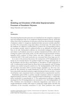
COMBINED PROBLEM
PARTICLE-ONLY
PROBLEMPROBLEM
FLUID-ONLY
=
+
Figure 8.1. Decomposition of the fluid/particle interaction (Zohdi [224]).
8.1 A model problem
We consider a sufficiently complex model problem comprising of agroup of nonintersecting
spherical particles (N
p
in total), each being small enough that their rotation with respect to
their mass centers is deemed insignificant. The equation of motion for the ith particle in the

system (Figure 8.1) is
m
i
¨
r
i
= 
tot
i
(r
1
, r
2
, ,r
N
p
), (8.1)
where r
i
is the position vector of the ith particle and 
tot
i
represents all forces acting on
particle i. In particular, 
tot
i
= 
drag
i
+ 

nf
i
+ 
con
i
+ 
fric
i
represents the forces due to
fluid drag, near-field interaction, interparticle contact forces, and frictional forces. Clearly,
under certain conditions one force may dominate over the others. However, this is generally
impossible to ascertain a priori, since the dynamics and coupling in the system may change
dramatically during the course of the flow process.
Remark. Throughout this chapter, boldface symbols indicate vectors or tensors. The
inner product of two vectors u and v is denoted by u · v. At the risk of oversimplification,
we ignore the distinction between second-order tensors and matrices. Furthermore, we
exclusively employ a Cartesian basis. Hence, if we consider the second-order tensor A
with its matrix representation [A], then the product of two second-order tensors A · B is
defined by the matrix product [A][B], with components of A
ij
B
jk
= C
ik
. The second-order
inner product of two tensors or matrices is A : B = A
ij
B
ij
= tr([A

T
][B]). Finally, the
divergence of a vector u is defined by ∇·u = u
i,i
, whereas for a second-order tensor A,
∇·A describes a contraction to a vector with the components A
ij,j
.
8.1.1 A simple characterization of particle/fluid interaction
We first consider drag force interactions between the fluid and the particles. The drag force
acting on an object in a fluid flow (occupying domain ω and outward surface normal n)is
defined as

drag
=

∂ω
σ
f
· n dA, (8.2)
where σ
f
is the Cauchy stress. For a Newtonian fluid, σ
f
is given by
σ
f
=−P
f
1 + λ

f
tr D
f
1 + 2µ
f
D
f
=−P
f
1 + 3κ
f
tr D
f
3
1 + 2µ
f
D

f
, (8.3)
where P
f
is the thermodynamic pressure, κ
f
= λ
f
+
2
3
µ

f
is the bulk viscosity, µ
f
is
05 book
2007/5/15
page 83
✐
✐
✐
✐
✐
✐
✐
✐
8.1. A model problem 83
the absolute viscosity, D
f
=
1
2
(∇
x
v
f
+ (∇
x
v
f
)

T
) is the symmetric part of the velocity
gradient, tr D
f
is the trace of D
f
, and D

f
= D
f
−
trD
f
3
1 is the deviatoric part of D
f
. The
stress is determined by solving the following coupled system of partial differential equations
(compressible Navier–Stokes):
Mass balance:
∂ρ
f
∂t
=−∇
x
· (ρ
f
v
f

),
Energy balance: ρ
f
C
f

∂θ
∂t
+ (∇
x
θ
f
) · v
f

= σ
f
:∇
x
v
f
+∇
x
· (K
f
·∇θ
f
) + ρ
f
z

f
,
Momentum balance: ρ
f

∂v
f
∂t
+ (∇
x
v
f
) · v
f

=∇
x
· σ
f
+ ρ
f
b
f
,
(8.4)
where, at a point, ρ
f
is the fluid density; v
f
is the fluid velocity; θ

f
is the fluid temperature;
C
f
is the fluid heat capacity; z
f
is the heat source per unit mass; K
f
is the thermal conduc-
tivity tensor, assumed to be isotropic of the form K
f
= K
f
1, K
f
being the scalar thermal
conductivity; and b
f
represents body forces per unit mass. The thermodynamic pressure is
given by an equation of state:
Z(P
f
,ρ
f
,θ
f
) = 0. (8.5)
The specific equation of state will be discussed later in the presentation.
The fluid domain will require spatial discretization with some type of mesh, for exam-
ple, usinga finite difference, finite volume, or finite elementmethod. Usually, it is extremely

difficult to resolve the flow in the immediate neighborhood of the particles, in particular
if there are several particles. However, if the primary interest is in the dynamics of the
particles, as it is in this work, an appropriate approach, which permits coarser discretization
of the fluid continuum, is to employ effective drag coefficients, for example, defined via
C
D
def
=
||
drag
i
||
1
2
ρ
f

ω
i
||v
f

ω
i
− v
i
||
2
A
i

, (8.6)
where (·)
ω
i
def
=
1
|ω
i
|

ω
i
(·)dω
i
is the volumetric average of the argument over the domain
occupied by the ith particle, v
f

ω
i
is the volumetric average of the fluid velocity, v
i
is
the velocity of the ith (solid) particle, and A
i
is the cross-sectional area of the ith (solid)
particle. For example, one possible way to represent the drag coefficient is with a piecewise
definition, as a function of the Reynolds number (Chow [44]):
• For 0 <Re≤ 1, C

D
=
24
Re
.
• For 1 <Re≤ 400, C
D
=
24
Re
0.646
.
• For 400 <Re≤ 3 × 10
5
, C
D
= 0.5.
• For 3 × 10
5
<Re≤ 2 ×10
6
, C
D
= 0.000366Re
0.4275
.
• For 2 × 10
6
<Re<∞, C
D

= 0.18.
Here, thelocal Reynolds number fora particle is Re
def
=
2b
i
ρ
f

ω
i
||v
f

ω
i
−v
i
||
µ
and b
i
is the radius
of the ith particle. The use of this simple concept makes it relatively straightforward to
05 book
2007/5/15
page 84
✐
✐
✐

✐
✐
✐
✐
✐
84 Chapter 8. Coupled particle/fluid interaction
account for the presenceofthesolid particles in the fluid by augmentingtheflowcalculations
with drag forces (Figure 8.1). Algorithmically speaking, one must compute the fluid flow
with reaction forces due to the presence of the particles. To this end, one can use the volu-
metric forces (b
f
) and heat sources (z
f
) within the fluid domain for this purpose by writing
ρ
f

∂v
f
∂t
+ (∇
x
v
f
) · v
f

=∇
x
· σ

f
+ ρ
f
b
f
,
b
f
= b
D
=−

drag
i
m
i
=−
C
D
1
2
ρ
f

ω
i
||v
f

ω

i
−v
i
||
2
A
i
m
i
d

d =
v
f

ω
i
−v
i
||v
f

ω
i
−v
i
||

,
ρ

f
C

∂θ
f
∂t
+ (∇
x
θ
f
) · v
f

= σ
f
:∇
x
v
f
+∇
x
· (K
f
·∇
x
θ
f
) + ρ
f
z

f
,
z
f
= z
D
= c
v
|b
D
· (v
f

ω
i
− v
i
)|,
(8.7)
where the drag force on the fluid, b
D
(per unit mass), is nonzero if its location coincides
with the particle domain and is zero otherwise. Here, z
D
is the heat source due to the rate
of work done by the drag force on the fluid.
43
Such source terms are easily projected onto a
finite difference or finite element grid.
44

This drag-based approach is designed to account
for particles in the fluid using a coarse mesh. In other words, the smallest (mesh) scale
allowable is that associated with the dimensions of the particles. Accordingly, we shall not
employ meshes smaller than the particle length scale when simulations are performed later.
Remark. More detailed analyses of fluid-particle interaction can be achieved in two
primary ways: (1) direct, brute-force, numerical schemes, treating the particles as part of
the fluid continuum (as another fluid or solid phase), and thus meshing them in a detailed
manner, or (2) with semi-analytical techniques, such as those based on approximation of
the interaction between the particles and the fluid, employing an analysis of the (interstitial)
fluid gaps using lubrication theory. For a concise review of recent developments in such
semi-analytical techniques, in particular methods that go beyond local analyses of flow
in a single fluid gap, using discrete network approximations, which account for multiple
hydrodynamic interactions, see Berlyand and Panchenko [30] and Berlyand et al. [31].
Although not employed here, discrete network approximations appear to be quite attractive
for possibly improving the description of the interaction between the particles and the fluid,
beyond a simple drag-based method (as adopted in this work), without resorting to detailed
numerical meshing.
8.1.2 Particle thermodynamics
Throughout the thermal analysis of the particles, we shall use relatively simple models.
Consistent with the particle-based philosophy, it is assumed that the temperature within
each particle is uniform (a lumped mass approximation). We remark that the validity of
assuming a uniform temperature within a particle is dictated by the Biot number. A small
Biot number indicates that such an approximation is reasonable. The Biot number for a
43
If the constant c
v
is not selected as unity, this can indicate endothermic or exothermic particle/fluid chemical
reactions.
44
If the particlesaresignificantly smaller than the meshspacing,thenthe drag forces associated withthe particles

are computed from the nearest node/particle center pair.
05 book
2007/5/15
page 85
✐
✐
✐
✐
✐
✐
✐
✐
8.1. A model problem 85
sphere scales with the ratio of particle volume (V ) to particle surface area (a
s
),
V
a
s
=
b
3
,
which indicates that auniform temperaturedistributionis appropriate, since theparticlesare,
by definition, small. Since it is assumed that the temperature fields are uniform within the
particles, the gradient of the temperature within the particle is zero, i.e., ∇θ = 0. Therefore,
a Fourier-type law for the heat flux will register a zero value, q =−K ·∇θ = 0.
Under these assumptions, we consider an energy balance, governing the interconver-
sions of mechanical, thermal, and chemical energy in a system, dictated by the first law of
thermodynamics. Accordingly, we require the time rate of change of the sum of the kinetic

energy (K) and stored energy (S) to be equal to the sum of the work rate (power, P) and
the net heat supplied (H):
d
dt
(K + S) = P +H, (8.8)
where we assume that the stored energy is composed solely of a thermal part, S = mCθ,
C being the heat capacity per unit mass. Consistent with the assumption that the particles
deform negligibly during impact, the amount of stored mechanical energy is deemed in-
significant. The kinetic energy is K =
1
2
mv · v. The mechanical power term is due to the
forces acting on a particle:
P =
dW
dt
= 
tot
· v. (8.9)
For the particles, it is assumed that a process of convection, for example, governed by
Newton’s law of cooling and thermal radiation according to a simple Stefan–Boltzmann
law, occurs. Accordingly, the first law reads
m
˙
v ·v + mC
˙
θ

 
d(K+S)

dt
= 
tot
· v

 
power=P
−h
c
a
s
(θ − θ
o
)

 
convection
+mc
v
|b
D
· (v
f

ω
− v)|

 
drag
−Ba

s
(θ
4
− θ
4
s
)

 
radiation
  
H
,
(8.10)
where θ
o
is the temperature of the ambient fluid, h
c
is the convection coefficient (using
Newton’s law of cooling), and θ
s
is the temperature of the far-field surface (for example,
a container surrounding the flow) with which radiative exchange is made. The Stefan–
Boltzmann constant is B = 5.67 ×10
−8
W
m
2
−K
;0≤  ≤ 1 is the emissivity, which indicates

how efficiently the surface radiates energy compared to a black-body (an ideal emitter);
0 ≤ h
c
is the convection coefficient (Newton’s law of cooling); and a
s
is the surface area
of a particle. It is assumed that the radiation exchange between the particles is negligible.
45
Because
dK
dt
= m
˙
v ·v = 
tot
·v = P, we obtain a simplified form of the first law,
dS
dt
= H,
and therefore Equation (8.10) becomes
mC
˙
θ =−h
c
a
s
(θ − θ
o
) + mc
v

|b
D
· (v
f

ω
− v)|−Ba
s
(θ
4
− θ
4
s
),
(8.11)
where θ
o
=θ
f

ω
is the local average of the surrounding fluid temperature.
Remark. To account for the convective exchange between the fluid and the particles,
we amend the source term in Equation (8.7) for the fluid to read
z
f
= z
D
= c
v

|b
f
· (v
f

ω
− v)|+
h
c
a
s
(θ − θ
o
)
m
. (8.12)
45
Various arguments for such an assumption can be found in the classical text of Bohren and Huffman [33].
05 book
2007/5/15
page 86
✐
✐
✐
✐
✐
✐
✐
✐
86 Chapter 8. Coupled particle/fluid interaction

If the fluid is “radiationally” thick, then we assume that no radiation enters the system from
the far field, namely, that Ba
s
θ
4
s
= 0 in Equation (8.11), and that any emission from the
particle gets absorbed by the fluid. Thus, in that situation, we can again amend the source
term to read
z
f
= z
D
= c
v
|b
f
· (v
f

ω
− v)|+
h
c
a
s
(θ − θ
o
) + Ba
s

θ
4
m
. (8.13)
Remark. We assume that various phenomena, such as near-field interaction, particle
contact, interparticle friction, and particle thermal sensitivity, are similar for the wet and
dry particulate flow problems, with the primary difference being that drag forces from the
surrounding fluid need to be determined via numerical discretization of the Navier–Stokes
equations, which is next.
46
8.2 Numerical discretization of the Navier–Stokes
equations
We now develop a fully implicit staggering scheme, in conjunction with a finite difference
discretization, to solve the coupled system. Generally, such schemes proceed, within a
discretized time step, by solving each field equation individually, allowing only the corre-
sponding primary field variable (ρ
f
, v
f
,orθ
f
) to be active. This effectively (momentarily)
decouples the system of differential equations. After the solution of each field equation,
the primary field variable is updated, and the next field equation is solved in a similar man-
ner, with only the corresponding primary variable being active. For accurate numerical
solutions, the approach requires small time steps, primarily because the staggering error
accumulates with each passing increment. Thus, such computations are usually computa-
tionally intensive.
First, let us consider a finite differencediscretizationof the derivatives in the governing
equations where, for brevity, we write (L indicates the time step counter, v

L
f
def
= v
f
(t),
v
L+1
f
def
= v
f
(t +t), etc.) for each finite difference node (i,j,k)
ρ
i,j,k,L+1
f
= ρ
i,j,k,L
f
− t

∇
x
· (ρ
f
v
f
)

i,j,k,L+1

,
Z(P
i,j,k,L+1
f
,ρ
i,j,k,L+1
f
,θ
i,j,k,L+1
f
) = 0,
θ
i,j,k,L+1
f
= θ
i,j,k,L
f
− t (∇
x
θ
f
· v
f
)
i,j,k,L+1
+

t
ρ
f

C
f
(σ
f
:∇
x
v
f
+∇
x
· (K
f
·∇
x
θ
f
) + ρ
f
z
f
)

i,j,k,L+1
,
v
i,j,k,L+1
f
= v
i,j,k,L
f

− t (∇
x
v
f
· v
f
)
i,j,k,L+1
+
t
ρ
f

∇
x
· σ
f
+ ρ
f
b
f

i,j,k,L+1
,
(8.14)
46
Clearly, the wetting of the particle surfaces, breaking of hydrodymanic films, etc., are nontrivial, but are
outside the scope of this introductory treatment.
05 book
2007/5/15

page 87
✐
✐
✐
✐
✐
✐
✐
✐
8.2. Numerical discretization of the Navier–Stokes equations 87
where the derivatives are computed by the following:

∂ρ
f
∂t

i,j,k,L
≈
ρ
f
(x
1
,x
2
,x
3
,t + t) − ρ
f
(x
1

,x
2
,x
3
,t)
t
=
ρ
i,j,k,L+1
f
− ρ
i,j,k,L
f
t
,
∇
x
· (ρ
f
v
f
) ≈
(ρ
f
v
f 1
)
i+1,j,k,L
− (ρ
f

v
f 1
)
i−1,j,k,L
2x
1
+
(ρ
f
v
f 2
)
i,j+1,k,L
− (ρ
f
v
f 2
)
i,j−1,k,L
2x
2
+
(ρ
f
v
f 3
)
i,j,k+1,L
− (ρ
f

v
f 3
)
i,j,k−1,L
2x
3
(8.15)
for the continuity equation;

ρ
f
C
f
∂θ
f
∂t

i,j,k,L
≈ ρ
i,j,k,L
f
C
f
(θ
i,j,k,L+1
f
−θ
i,j,k,L
f
)

t
,
(ρ
f
C
f
∇
x
θ
f
· v
f
)
i,j,k,L
≈ ρ
i,j,k,L
f
C
f
×

v
i,j,k,L
f 1
θ
i+1,j,k,L
f
−θ
i−1,j,k,L
f

2x
1
+ v
i,j,k,L
f 2
θ
i,j+1,k,L
f
−θ
i,j−1,k,L
f
2x
2
+ v
i,j,k,L
f 3
θ
i,j,k+1,L
f
−θ
i,j,k−1,L
f
2x
3

,
(σ
f
:∇
x

v
f
)
i,j,k,L
≈ σ
i,j,k,L
f 11
v
i+1,j,k,L
f 1
−v
i−1,j,k,L
f 1
2x
1
+σ
i,j,k,L
f 22
v
i,j+1,k,L
f 2
−v
i,j−1,k,L
f 2
2x
2
+ σ
i,j,k,L
f 33
v

i,j,k+1,L
f 3
−v
i,j,k−1,L
f 3
2x
3
+σ
i,j,k,L
f 12

v
i,j+1,k,L
f 1
−v
i,j−1,k,L
f 1
2x
2
+
v
i+1,j,k,L
f 2
−v
i−1,j,k,L
f 2
2x
1

+σ

i,j,k,L
f 23

v
i,j,k+1,L
f 2
−v
i,j,k−1,L
f 2
2x
3
+
v
i,j+1,k,L
f 3
−v
i,j−1,k,L
f 3
2x
2

+σ
i,j,k,L
f 31

v
i+1,J,k,L
f 3
−v
i−1,j,k,L

f 3
2x
1
+
v
i,j,k+1,L
f 1
−v
i,j,k−1,L
f 1
2x
3

,
(∇
x
·(K
f
·∇
x
θ
f
))
i,j,k,L
≈K
i,j,k,L
θ
i+1,j,k,L
f
−2θ

i,j,k,L
f
+θ
i−1,j,k,L
f
x
2
1
+K
i,j,k,L
f
θ
i,j+1,k,L
f
−2θ
i,j,k,L
f
+θ
i,j−1,k,L
f
x
2
2
+K
i,j,k,L
f
θ
i,j,k+1,L
f
−2θ

i,j,k,L
f
+θ
i,j,k−1,L
f
x
2
3
(8.16)
05 book
2007/5/15
page 88
✐
✐
✐
✐
✐
✐
✐
✐
88 Chapter 8. Coupled particle/fluid interaction
for the balance of energy; and

∂v
f 1
∂t

i,j,k,L
≈
v

i,j,k,L+1
f 1
− v
i,j,k,L
f 1
t
,

∂v
f 2
∂t

i,j,k,L
≈
v
i,j,k,L+1
f 2
− v
i,j,k,L
f 2
t
,

∂v
f 3
∂t

i,j,k,L
≈
v

i,j,k,L+1
f 3
− v
i,j,k,L
f 3
t
,
((∇
x
v
f
) · v
f
)
i,j,k,L
≈ v
i,j,k,L
f 1
v
i+1,j,k,L
f 1
− v
i−1,j,k,L
f 1
2x
1
+v
i,j,k,L
f 2
v

i,j+1,k,L
f 1
− v
i,j−1,k,L
f 1
2x
2
+ v
i,j,k,L
f 3
v
i,j,k+1,L
f 1
− v
i,j,k−1,L
f 1
2x
3
+v
i,j,k,L
f 1
v
i+1,j,k,L
f 2
− v
i−1,j,k,L
f 2
2x
1
+ v

i,j,k,L
f 2
v
i,j+1,k,L
f 2
− v
i,j−1,k,L
f 2
2x
2
+v
i,j,k,L
f 3
v
i,j,k+1,L
f 2
− v
i,j,k−1,L
f 2
2x
3
+ v
i,j,k,L
f 1
v
i+1,j,k,L
f 3
− v
i−1,j,k,L
f 3

2x
1
+v
i,j,k,L
f 2
v
i,j+1,k,L
f 3
−v
i,j−1,k,L
f 3
2x
2
+v
i,j,k,L
f 3
v
i,j,k+1,L
f 3
−v
i,j,k−1,L
f 3
2x
3
,
(∇
x
· σ
f
)

i,j,k,L
≈

σ
i+1,j,k,L
f 11
− σ
i−1,j,k,L
f 11
2x
1
+
σ
i,j+1,k,L
f 12
− σ
i,j−1,k,L
f 12
2x
2
+
σ
i,j,k+1,L
f 13
− σ
i,j,k−1,L
f 13
2x
3


e
1
+

σ
i+1,j,k,L
f 21
− σ
i−1,j,k,L
f 21
2x
1
+
σ
i,j+1,k,L
f 22
− σ
i,j−1,k,L
f 22
2x
2
+
σ
i,j,k+1,L
f 23
− σ
i,j,k−1,L
f 23
2x
3


e
2
+

σ
i+1,j,k,L
f 31
− σ
i−1,j,k,L
f 31
2x
1
+
σ
i,j+1,k,L
f 32
− σ
i,j−1,k,L
f 32
2x
2
+
σ
i,j,k+1,L
f 33
− σ
i,j,k−1,L
f 33
2x

3

e
3
(8.17)
for thebalance of linear monentum. The discretized system is formulated next as an implicit
time-stepping scheme within each time step L, whereby (1) one solves for the density,
assuming the thermal and velocity fields fixed, (2) one solves for the temperature, assuming
the density and velocity fields fixed, and then (3) one solves for the velocity, assuming
the density and thermal fields fixed. Below, we formulate such a system, with an iterative
counter K (within a time step), for each finite difference node:
05 book
2007/5/15
page 89
✐
✐
✐
✐
✐
✐
✐
✐
8.3. Numerical discretization of the particle equations 89
ρ
i,j,k,L+1,K
f
= ρ
i,j,k,L
f
− t


∇
x
· (ρ
f
v
f
)
f

i,j,k,L+1,K−1
,
Z

P
i,j,k,L+1,K−1
f
,ρ
i,j,k,L+1,K
f
,θ
i,j,k,L+1,K−1
f

= 0,
θ
i,j,k,L,K
f
= θ
i,j,k,L

f
− t (∇
x
θ
f
· v
f
)
i,j,k,L+1,K−1
+

t
ρ
f
C
f

σ
f
:∇
x
v
f
+∇
x
· (K
f
·∇
x
θ

f
) + ρ
f
z
f


i,j,k,L+1,K−1
,
v
i,j,k,L+1,K
f
= v
i,j,k,L
f
−t (∇
x
v
f
· v
f
)
i,j,k,L+1,K−1
+

t
ρ
f

∇

x
· σ
f
+ρ
f
b
f


i,j,k,L+1,K−1
.
(8.18)
In an abstract setting, we have
A
f 1

ρ
L+1,K
f
,θ
L+1,K−1
f
, v
L+1,K−1
f

= F
f 1

ρ

L+1,K−1
f
,θ
L+1,K−1
f
, v
L+1,K−1
f
,

(CONTINUITY),
A
f 2

ρ
L+1,K
f
,θ
L+1,K
f
, v
L+1,K−1
f

= F
f 2

ρ
L+1,K
f

,θ
L+1,K−1
f
, v
L+1,K−1
f
,

(ENERGY),
A
f 3

ρ
L+1,K
f
,θ
L+1,K
f
, v
L+1,K
f

= F
f 3

ρ
L+1,K
f
,θ
L+1,K

f
, v
L+1,K−1
f
,

(MOMENTUM),
(8.19)
where only the underlined variable is active (to be solved for) in the corresponding differ-
ential equation, and where K is an iteration counter.
8.3 Numerical discretization of the particle equations
As for the dry particulate cases, for the time discretization of the acceleration terms in the
equations of motion (Equation (8.1)), for each particle, we write
¨
r
L+1
≈
˙
r
L+1
−
˙
r
L
t
≈
r
L+1
−r
L

t
−
˙
r
L
t
≈
r
L+1
− r
L
t
2
−
˙
r
L
t
, (8.20)
which collapses to the familiar difference stencil of
¨
r
L+1
≈
r
L+1
−2r
L
+r
L−1

(t)
2
when the time
step size is uniform. Inserting this into m
¨
r = 
tot
(r) leads to
r
L+1,K
≈
t
2
m


tot
(r
L+1,K−1
)

+

r
L
+ t
˙
r
L


. (8.21)
05 book
2007/5/15
page 90
✐
✐
✐
✐
✐
✐
✐
✐
90 Chapter 8. Coupled particle/fluid interaction
For the thermal behavior, aftertemporal integration with thepreviously used finite difference
time step (for the fluid), we have from Equation (8.20)
θ(t + t) =
mC
mC + h
c
a
s
t
θ(t) −
tBa
s

mC + h
c
a
s

t

θ
4
(t +t) − θ
4
s

+
mc
v
t|b
D
· (v
f

ω
− v)|
mC + h
c
a
s
t
+
h
c
a
s
tθ
o

mC + h
c
a
s
t
.
(8.22)
This implicit nonlinear equation for θ, for each particle, is recast as
θ
L+1,K
=
mC
mC + h
c
a
s
t
θ
L
−
tBa
s

mC + h
c
a
s
t

(θ

L+1,K−1
)
4
− θ
4
s

+
mc
v
t|b
D
· (v
L+1,K
f

ω
− v
L+1,K
)|
mC + h
c
a
s
t
+
h
c
a
s

tθ
o
mC + h
c
a
s
t
(8.23)
and is added into the fixed-point scheme with the equations of momentum balance and the
equations governing the fluid mechanics. Concisely, the equations for the particle mechanics
problem can be addressed in an abstract setting, whereby one solves for the particle positions,
assuming the thermal fields fixed,
A
p1
(r
L+1,K
,θ
L+1,K−1
) = F
p1
(r
L+1,K−1
,θ
L+1,K−1
), (8.24)
and then one solves for the thermal fields, assuming the particle positions fixed,
A
p2
(r
L+1,K

,θ
L+1,K
) = F
p2
(r
L+1,K
,θ
L+1,K−1
). (8.25)
Both of these equations, and the equations for the fluid, are solved simultaneously with an
adaptive multifield staggering scheme, which we shall discuss shortly.
Remark. In order to determine the thermal state of the particles when impact-induced
reactions are significant, we shall decompose the heat generation and heat transfer processes
into two stages. Stage I describes the extremely short time interval when impact occurs,
δt  t, and accounts for the effects of chemical reactions, which are relevant in cer-
tain applications, and energy release due to mechanical straining. Stage II accounts for
the postimpact behavior involving convective and radiative effects, as discussed earlier.
As before, we consider an energy balance, governing the interconversions of mechanical,
thermal, and chemical energy in a system, dictated by the first law of thermodynamics,
d
dt
(K + S) = P + H, with the previous assumptions leading to
dS
dt
= H. For Stage I, the
primary source of heat is the chemical reactions that occur upon impact due to the presence
of a reactive layer. The chemical reaction energy is defined as
δH
def
=


t+δt
t
H dt. (8.26)
The first law can be rewritten for the temperature at time = t +δt as
θ(t + δt) = θ(t)+
δH
mC
. (8.27)
05 book
2007/5/15
page 91
✐
✐
✐
✐
✐
✐
✐
✐
8.4. An adaptive staggering solution scheme 91
The energy released from the reactions is assumed to be proportional to the amount of the
fluid substance (for example, a gas) available to be compressed in the contact area between
the particles. A typical, ad hoc approximation in combustion processes is to write, for
example, a linear relation, with a saturation (limiting) value (ξ),
δH ≈ ξ min

|
I
n

|
I
∗
n
, 1

πb
2
, (8.28)
where ξ isthereactionconstant (energy per unit area [J/m
2
]), I
∗
n
is a normalization parameter,
and b is the particle radius. For details on a variety of such relations, see, for example,
Schmidt [172]. For the particle sizes and material properties of interest, the term
δH
mC
in
Equation (8.27) indicates that
δθ
def
= θ(t + δt) −θ(t) =
δH
mC
∝
ξ
ρCb
. (8.29)

Thus, when values of ξ are chosen such that
ξ
ρCb
 1, this will generate asignificant amount
of heat.
47
Thereafter (Stage II, postimpact), it is assumed that a process of convection, for
example, governed by Newton’s law of cooling and radiation according to a simple Stefan–
Boltzmann law, occurs. Since δt  t we assign
θ
L
= θ(t +δt) = θ(t)+
δH
mC
and replace
θ
L
with it in Equation (8.23) to obtain
θ(t + t) =
mC
mC + h
c
a
s
t
θ(t) −
tBa
s

mC + h

c
a
s
t

θ
4
(t +t) − θ
4
s

+
mc
v
t|b
D
· (v
f

ω
− v)|
mC + h
c
a
s
t
+
h
c
a

s
tθ
o
mC + h
c
a
s
t
.
(8.30)
8.4 An adaptive staggering solution scheme
We now develop a temporally adaptive staggering scheme by extending the approach pre-
sented earlier. Let us denote the entire coupled system as A(w
L+1
) = F , where w is a
multifield vector that represents the particle positions (r) , the particle temperatures (θ),
the nodal fluid velocities (v
f
), and the temperatures (θ
f
), i.e., w = (r,θ,v
f
,θ
f
).Itis
convenient to write
A(w
L+1
) − F = G(w
L+1

) − w
L+1
+ R = 0, (8.31)
where R is a remainder term that does not depend on the solution, i.e., R = R(w
L+1
).A
straightforward iterative scheme can be written as
w
L+1,K
= G(w
L+1,K−1
) + R, (8.32)
where K = 1, 2, 3, is the index of iteration within time step L + 1. The convergence
of such a scheme depends on the characteristics of G. Namely, a sufficient condition for
47
By construction, this model has increased heat production, via δH,asκ increases.
05 book
2007/5/15
page 92
✐
✐
✐
✐
✐
✐
✐
✐
92 Chapter 8. Coupled particle/fluid interaction
convergence is that G is a contraction mapping for all w
L+1,K

, K = 1, 2, 3 In order to
investigate this further, we define the staggering error as E
L+1,K
= w
L+1,K
−w
L+1
. A nec-
essary restriction for convergence is iterative self-consistency, i.e., the “exact” (staggering
error–free) solution must be represented by the scheme G(w
L+1
) + R = w
L+1
. Enforc-
ing this restriction, a sufficient condition for convergence is the existence of a contraction
mapping of the form
||E
L+1,K
||
def
=||w
L+1,K
−w
L+1
||=||G(w
L+1,K−1
) −G(w
L+1
)|| ≤ η||w
L+1,K−1

−w
L+1
||,
(8.33)
where, if η<1 for each iteration K, then E
L+1,K
→ 0 for any arbitrary starting value
w
L+1,K=0
as K →∞. This contraction condition is sufficient, but not necessary, for
convergence. For example, if we isolate the equation for the dynamics of the particles,
r
L+1,K
≈
t
2
m


tot
(r
L+1,K−1
)


 
G(r
L+1,K−1
)
+


r
L
+ t
˙
r
L


 
R
, (8.34)
we observe that convergence is restricted by η ∝ EIG(G) ∝
t
2
m
. Thus, decreasing the
time step size improves the convergence; however, we want to simultaneously maximize
the time step sizes to decrease overall computing time while still meeting an error tolerance.
In order to achieve this goal, we follow the approach provided earlier where (1) one approx-
imates η ≈ S(t)
p
(S is a constant) and (2) one assumes that the error within an iteration
behaves approximately according to (S(t)
p
)
K
||E
L+1,0
||=||E

L+1,K
||, K = 1, 2, ,
where ||E
L+1,0
|| is the initial norm of the iterative error and S is a function intrinsic to the
system.
48
Our goal is to meet an error tolerance in exactly a preset number of iterations. To
this end, we write this in the approximate form (S(t
tol
)
p
)
K
d
||E
L+1,0
|| = TOL, where TOL
is a tolerance and K
d
is the desired number of iterations.
49
If the error tolerance is not met
in the desired number of iterations, the contraction constant η is too large. Accordingly, we
can solve for a new smaller step size, under the assumption that S is constant:
50
t
tol
= t





TOL
||E
L+1,0
||

1
pK
d

||E
L+1,K
||
||E
L+1,0
||

1
pK



. (8.35)
The assumption that S is constant is not critical, since the time steps are to be recursively
refined and unrefined repeatedly. Clearly, the previous expression can also be used for time
step enlargement if convergence ismet in fewer than K
d
iterations. Time stepsize adaptivity

is paramount, since the flow’s dynamics can dramatically change over the course of time,
requiring radically different time step sizes for a preset level of accuracy. However, we
must respect an upper bound dictated by the discretization error, i.e., t ≤ t
lim
. In order
to couple this to the multifield computations, we define the normalized errors within each
48
For the class of problems under consideration, due to the quadratic dependency on t, p ≈ 2.
49
Typically, K
d
is chosen to be between five and ten iterations.
50
In the definition of the error, since the “true” solution at a time step, w
L+1
, is unknown, we use the most
current value of the solution, w
L+1,K
; thus, the error is to be interpreted as the relative error.
05 book
2007/5/15
page 93
✐
✐
✐
✐
✐
✐
✐
✐

8.4. An adaptive staggering solution scheme 93
time step:
E
rK
def
=
||r
L+1,K
− r
L+1,K−1
||
||r
L+1,K
− r
L
||
and E
θK
def
=
||θ
L+1,K
− θ
L+1,K−1
||
||θ
L+1,K
− θ
L
||

(8.36)
for the particles (summing over all particles) and
ˆ
E
r
f
K
def
=
||v
L+1,K
f
− v
L+1,K−1
f
||
||v
L+1,K
f
− v
L
f
||
and
ˆ
E
θ
f
K
def

=
||θ
L+1,K
f
− θ
L+1,K−1
f
||
||θ
L+1,K
f
− θ
L
f
||
(8.37)
for the fluid (summing over all of the finite difference nodes). One can interpret these error
metrics as the ratio of the staggering error to the change in the actual solution (from time
step to time step). We now combine all of these (normalized) error metrics (ratios) into one
single measure:
E
tot,K
=
w
1
E
rK
+ w
2
E

θK
+ w
3
ˆ
E
r
f
K
+ w
4
ˆ
E
θ
f
K
w
1
+ w
2
+ w
3
+ w
4
, (8.38)
where the w
i
’s are weights. The overall algorithm is given as Algorithm 8.1. The purpose
of the algorithm is to deliver solutions where the coupling is resolved in an iterative manner
by the recursive staggered solution of the various field equations, constraints, etc. The
incomplete coupling error is controlled by adaptively adjusting the time step sizes, while

the temporal discretization accuracy dictates the upper limit on the time step size (t
lim
).
Remark. As before, inAlgorithm 8.1, atthe implementation level, normalized (nondi-
mensional) error measures were used. As with the unnormalized case, one approximates
the error within an iteration to behave according to
(S(t)
p
)
K
||r
L+1,1
− r
L+1,0
||
||r
L+1,0
− r
L
||

 
E
0
=
||r
L+1,K
− r
L+1,K−1
||

||r
L+1,K
− r
L
||

 
E
K
, (8.39)
where the normalized measures characterize the ratio of the iterative (staggering) error
within a time step to the difference in solutions between time steps. Since both ||r
L+1,0
−
r
L
|| ≈ O(t) and ||r
L+1,K
− r
L
|| ≈ O(t) are of the same order, the use of normalized
or unnormalized measures makes little difference in rates of convergence. However, the
normalized measures are preferred since they have a clearer interpretation.
Remark. We remark that the forces needed to compute terms in the coefficient of
restitution e, for example, E
in
, E
jn
, and D
ij

, are obtained by using the most current known
values of the 
i
’s during the iterative solution process. In other words, the interaction
forces are updated during the iterations, within a time step, based on the most current known
positions of the particles. This process includes checking whether ||r
i
− r
j
|| ≤ b
i
+ b
j
,
which is a criterion for contact between particles.
Remark. For the fluid, notice that all of the contraction factors in Equation (8.19)
scale as
t
h
and
t
h
2
(classical stability terms).
Remark. The result in Equation (7.51) provides a rough guide as to the selection of
the exponent (p) for the overallsystem (when many different types ofequations are present).
The exponent p is approximately the sum of the product of each field equation that contains
a numerical time derivative and the order of the corresponding time differentiation (first
05 book
2007/5/15

page 94
✐
✐
✐
✐
✐
✐
✐
✐
94 Chapter 8. Coupled particle/fluid interaction
(0) GLOBAL FIXED-POINT ITERATION (SET i = 1 AND K = 0):
(1) COMPUTE FLUID SOLUTION (FOR EACH NODE): (v
f
,ρ
f
,θ
f
)
L+1,K
(FREEZING PARTICLE POSITIONS);
(2) IF i>N
p
, THEN GO TO (4);
(3) IF i ≤ N
p
, THEN (FREEZING FLUID VARIABLES)
(a) COMPUTE POSITION: r
L+1,K
i
=

t
2
m
i


tot
i
(r
L+1,K−1
)

+ r
L
i
+ t
˙
r
L
i
;
(b) COMPUTE TEMPERATURE:
θ
L+1,K
i
=
mC
mC + h
c
a

s
t
θ
L+1,K−1
i
−
tBa
s

mC + h
c
a
s
t

(θ
L+1,K−1
i
)
4
− θ
4
s

+
h
c
a
s
tθ

o
mC + h
c
a
s
t
+
mc
v
t|b
D
· (v
L+1,K
f

ω
i
− v
L+1,K
)|
mC + h
c
a
s
t
;
(c) GO TO (2) AND NEXT FLOW PARTICLE (i = i +1);
(4) ERROR MEASURES:
(a) E
rK

def
=

N
p
i=1
||r
L+1,K
i
− r
L+1,K−1
i
||

N
p
i=1
||r
L+1,K
i
− r
L
i
||
, E
θK
def
=

N

p
i=1
||θ
L+1,K
i
− θ
L+1,K−1
i
||

N
p
i=1
||θ
L+1,K
i
− θ
L
i
||
,
ˆ
E
r
f
K
def
=
||v
L+1,K

f
− v
L+1,K−1
f
||
||v
L+1,K
f
− v
L
f
||
,
ˆ
E
θ
f
K
def
=
||θ
L+1,K
f
− θ
L+1,K−1
f
||
||θ
L+1,K
f

− θ
L
f
||
;
(b) E
tot,K
=
w
1
E
rK
+ w
2
E
θK
+ w
3
ˆ
E
rK
+ w
4
ˆ
E
θK
w
1
+ w
2

+ w
3
+ w
4
,
TOL
tot
=
w
1
TOL
r
+ w
2
TOL
θ
+ w
3
TOL
r
f
+ w
4
TOL
θ
f
w
1
+ w
2

+ w
3
+ w
4
;
(c) 
K
def
=




TOL
tot
E
tot,0

1
pK
d

E
tot,K
E
tot,0

1
pK




;
(5) IF TOLERANCE MET (E
tot,K
≤ 1) AND K<K
d
, THEN
(a) INCREMENT TIME: t = t + t;
(b) CONSTRUCT NEW TIME STEP: t = 
K
t;
(c) SELECT MINIMUM t = min(t
lim
,t)AND GO TO (0);
(6) IF TOLERANCE NOT MET (E
tot,K
> TOL) AND K = K
d
, THEN
(a) CONSTRUCT NEW TIME STEP: t = 
K
t;
(b) RESTART AT TIME = t AND GO TO (0).
Algorithm 8.1
05 book
2007/5/15
page 95
✐
✐

✐
✐
✐
✐
✐
✐
8.5. A numerical example 95
order, second order, etc.), divided by the sum of the number of equations using numerical
time derivatives in the system. Explicitly,
p ≈

N
i=1
O
i
N
, (8.40)
where N is the number of field equations where a numerical derivative was used and O
i
is
the order of the time differentiation (first order, second order, etc.) of the individual field
equation i.
Remark. An alternative and more severe way to measure the error is to define
“violation ratios,” i.e., the measure of which field is relatively more in error, compared to
its corresponding tolerance, via Z
K
def
= max(z
rK
,z

θK
, ˆz
vK
, ˆz
θ
f
K
), where
z
rK
def
=
E
rK
TOL
r
and z
θK
def
=
E
θK
TOL
θ
(8.41)
and
ˆz
vK
def
=

ˆ
E
vK
TOL
v
and ˆz
θ
f
K
def
=
ˆ
E
θK
TOL
θ
f
,
(8.42)
and then a minimum scaling factor 
K
def
= min(φ
rK
,φ
θK
,
ˆ
φ
vK

,
ˆ
φ
θ
f
K
), where, for the parti-
cles
φ
rK
def
=



TOL
r
E
r0

1
pK
d

E
rK
E
r0

1

pK


,φ
θK
def
=



TOL
θ
E
θ0

1
pK
d

E
θK
E
θ0

1
pK


(8.43)
and for the fluid

ˆ
φ
vK
def
=



ˆ
TOL
v
ˆ
E
v0

1
pK
d

ˆ
E
vK
ˆ
E
v0

1
pK



,
ˆ
φ
θ
f
K
def
=





ˆ
TOL
θ
ˆ
E
θ0

1
pK
d

ˆ
E
θ
f
K
ˆ

E
θ
f
0

1
pK




.
(8.44)
However, in such an approach, if the individual field withthemaximum error is used fortime
step adaptivity, we need to specifically use the corresponding convergence exponent (p) for
the selected field’s temporal discretization. If the equations of dynamic equilibrium of the
particles are the field chosen, then p = 2. If the equations of thermodynamic equilibrium
of the particles are the field chosen, then p = 1. If the equations of dynamic equilibrium of
the fluid are the field chosen, then p = 1. If the equations of thermodynamic equilibrium
of the fluid are the field chosen, then p = 1. However, this approach has some major
drawbacks when many disparate fields are present. Specifically, when the maximum error
measure oscillates from field to field within a time step or abruptly from time step to time
step, convergence becomes quite difficult. Using the combined metric (Equation (8.38)) is
more stable and, thus, preferred.
8.5 A numerical example
As a model problem, we considered a cubical representative volume of a particle-laden fluid
flow (Figure 8.2). The classical random sequential addition algorithm was used to initially
place nonoverlapping spherical particles into the domain of interest (Widom [200]). This