An Introduction to Modeling and Simulation of Particulate Flows Part 7 docx

05 book
2007/5/15
page 96
✐
✐
✐
✐
✐
✐
✐
✐
96 Chapter 8. Coupled particle/fluid interaction
Figure 8.2. A representative volume element extracted from a flow (Zohdi [224]).
algorithm was adequate for the volume fraction ranges of interest (under 30%), since the
limit of the method is on the order of 38%.
Any particles that exited a boundary were given the same velocity (now incoming)
on the opposite boundary. Periodicity conditions were used to generate any numerical
derivatives for finite difference stencils that extended beyond the boundary. Clearly, under
these conditions the group velocity of the particles will tend toward the velocity of the
(“background”) fluid specified (controlled) on the boundary.
A Boussinesq-type (perturbation from an ideal gas) relation, adequate to describe
dense gases, and fluids, was used for the equation of state, stemming from
ρ
f
≈ ρ
o
(θ
o
,P
o
) +

∂ρ
f
∂P
f




θ
P
f
+
∂ρ
f
∂θ
f




P
f
θ
f
, (8.45)
where ρ
o
, θ
o
, P

o
are reference values, P
f
= P
f
−P
o
, and θ
f
= θ
f
−θ
o
. We define the
thermal expansion as
ζ
θ
def
=−
1
ρ
f
∂ρ
f
∂θ
f





P
f
=
1
V
f
∂V
f
∂θ
f





P
f
(8.46)
and the bulk (compressibility) modulus by
ζ
com
def
=−V
f
∂P
f
∂V
f





θ
f
= ρ
f
∂P
f
∂ρ
f





θ
f
, (8.47)
yielding the desired result
ρ
f
≈ ρ
o

1 − ζ
θ
θ
f
+
1

ζ
com
P
f

, (8.48)
leading to
P
f
≈ P
o
+ ζ
com

ρ
f
ρ
o
− 1 + ζ
θ
θ
f

, (8.49)
05 book
2007/5/15
page 97
✐
✐
✐

✐
✐
✐
✐
✐
8.5. A numerical example 97
where O(ζ
θ
) ≈ 10
−7
/
◦
K and 10
5
Pa < O(ζ
com
)<10
10
Pa. The viscosity is assumed to
behave according to the well-known relation
µ
f
µ
r
= e
c(
θ
r
θ
f

−1)
, (8.50)
where µ
r
is a reference viscosity, θ
r
is a reference temperature, and c is a material constant.
As before, we introduce the following (per unit mass
2
) decompositions for the key near-field
parameters, for example, for the force imparted on particle i by particle j and vice versa:
51
• α
1ij
= α
1
m
i
m
j
,
• α
2ij
= α
2
m
i
m
j
.

One should expect two primary trends:
• Larger particles are more massive and can impact one another without significant
influence from the surrounding fluid. In other words, the particles can “plow”through
the fluid and make contact. This makes this situation more thermally volatile, due to
the resulting chemical release at contact.
• Smaller particles are more sensitive to the surrounding fluid, and the drag ameliorates
the disparity in velocities, thus minimizing the interparticle impact. Thus, these types
of flows are less thermally sensitive.
Obviously, in such a model, the number of parameters, even though they are not
ad hoc, is large. Thus, corresponding parameter studies would be enormous. This is not
the objective of this book. Accordingly, we have taken nominal parameter values that fall
roughly in the middle ofmaterialdataranges to illustrate the basic approach. The parameters
selected for the simulations were as follows:
52
• a (normalized) domain size of 1 m ×1m×1m;
• 200 particles randomly distributed in the domain and all started from rest;
• the particle radii randomly distributed in the range b = 0.05(1 +±0.25) m, resulting
in approximately 11% of the volume being occupied by the particles;
• an initial velocity of v
f
= (1m/s, 0m/s, 0m/s) assigned to the fluid and periodic
boundary conditions used;
• viscosity parameters µ
r
= 0.05 N − s/m
2
and c = 5, for the equation of state
(Boussinesq-type model), and the same thermal relation assumed for the bulk viscos-
ity, namely,
κ

f
κ
r
= e
c(
θ
r
θ
f
−1)
, κ
r
= 0.8µ
r
;
53
• a uniform initial particle temperature of θ = 293.13
◦
K;
• a uniform initial fluid interior temperature of θ
f
= 293.13
◦
K serving as the boundary
conditions for the domain;
• a particle heat capacity of C = 1000 J/(kg
◦
K);
51
Alternatively, if the near-fields are related to the amount of surface area, this scaling could be done per unit

area.
52
No gravitational effects were considered.
53
In order to keep the analysis general, we do not enforce the Stokes condition, namely, κ
f
= 0.
05 book
2007/5/15
page 98
✐
✐
✐
✐
✐
✐
✐
✐
98 Chapter 8. Coupled particle/fluid interaction
• a fluid heat capacity of C
f
= 2500 J/(kg
◦
K);
• a fluid conductivity of K
f
= 1.0Jm
2
/(s kg
◦

K);
• a radiative particle emissivity of  = 0.05;
• near-field parameters for the particles of
α
1
= 0.1, α
2
= 0.01, β
1
= 1, β
2
= 2;
• restitution impact coefficients of e
−
= 0.1 (the lowerbound), e
o
= 0.2, θ
∗
= 3000
◦
K
(thermal sensitivity coefficient), v
∗
= 10 m/s;
• a coefficient of static friction of µ
s
= 0.5 and a coefficient of dynamic friction of
µ
d
= 0.2;

• a reaction coefficient of ξ = 10
9
J/m
2
and a reaction impact parameter of I
∗
= 10
3
N;
• a heat-drag coefficient of c
v
= 1;
• a convective heat transfer coefficient of h
c
= 10
3
J/(sm
2 ◦
K);
• a bulk fluid (compressibility) modulus of ζ
com
= 10
6
Pa, a reference pressure of P
o
=
101300 Pa (1 atm), a reference density of ρ
o
= 1000 kg/m
3

, a reference temperature
of θ
o
= 293.13
◦
K, and a thermal expansion coefficient of ζ
θ
= 10
−7◦
(K)
−1
;
• a particle density of ρ = 2000 kg/m
3
.
The discretization parameters selected were
•a10× 10 × 10 finite difference mesh (with a spacing of 0.1 m) for the numerical
derivatives (on the order of the particle size);
• a simulation time of 1 s;
• an initial time step size of 10
−6
s;
• an upper limit for the time step size of 10
−2
s;
• a lower limit for the time step size of 10
−12
s;
• a target number of internal fixed-point iterations of K
d

= 5;
• a (percentage) iterative (normalized) relative error tolerance within a time step set to
TOL
1
= TOL
2
= TOL
3
= TOL
4
= 10
−3
.
8.6 Discussion of the results
For this system, the Reynolds number, based on the mean particle diameter and initial sys-
tem parameters, was Re
def
=
ρ
o
2bv
o
µ
o
≈ 4010. The plots in Figures 8.3–8.6 illustrate the
system behavior with and without near-fields. There is significant heating due to interpar-
ticle collisions when near-fields are present. The presence of near-fields causes particle
trajectories due to mutual attraction and repulsion, and particles to make contact frequently.
05 book
2007/5/15

page 99
✐
✐
✐
✐
✐
✐
✐
✐
8.6. Discussion of the results 99
X
0
0.2
0.4
0.6
0.8
1
Y
0.2
0.4
0.6
0.8
Z
0.2
0.4
0.6
0.8
600
580
560

540
520
500
480
460
440
420
400
380
360
340
320
300
X
0
0.2
0.4
0.6
0.8
1
Y
0.2
0.4
0.6
0.8
Z
0.2
0.4
0.6
0.8

600
580
560
540
520
500
480
460
440
420
400
380
360
340
320
300
X
0
0.2
0.4
0.6
0.8
1
Y
0.2
0.4
0.6
0.8
Z
0.2

0.4
0.6
0.8
600
580
560
540
520
500
480
460
440
420
400
380
360
340
320
300
X
0
0.2
0.4
0.6
0.8
1
Y
0.2
0.4
0.6

0.8
Z
0.2
0.4
0.6
0.8
600
580
560
540
520
500
480
460
440
420
400
380
360
340
320
300
X
0
0.2
0.4
0.6
0.8
1
Y

0.2
0.4
0.6
0.8
Z
0.2
0.4
0.6
0.8
600
580
560
540
520
500
480
460
440
420
400
380
360
340
320
300
X
0
0.2
0.4
0.6

0.8
1
Y
0.2
0.4
0.6
0.8
Z
0.2
0.4
0.6
0.8
600
580
560
540
520
500
480
460
440
420
400
380
360
340
320
300
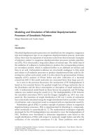
Figure 8.3. With near-fields: Top to bottom and left to right, the dynamics of the
particulate flow. Blue (lowest) indicates a temperature of approximately 300

◦
K, while red
(highest) indicates a temperature of approximately 600
◦
K. The arrows on the particles
indicate the velocity vectors (Zohdi [224]).
05 book
2007/5/15
page 100
✐
✐
✐
✐
✐
✐
✐
✐
100 Chapter 8. Coupled particle/fluid interaction
-0.1
0
0.1
0.2
0.3
0.4
0.5
0.6
0 0.2 0.4 0.6 0.8 1 1.2
AVERAGE PARTICLE VELOCITIES (m/s)
TIME/TIME LIMIT
VPX

VPY
VPZ
290
300
310
320
330
340
350
0 0.2 0.4 0.6 0.8 1 1.2
AVERAGE PARTICLE TEMPERATURE (Kelvin)
TIME/TIME LIMIT
Figure 8.4. Withnear-fields: Theaverage velocity and temperature of the particles
(Zohdi [224]).
-0.1
0
0.1
0.2
0.3
0.4
0.5
0.6
0 0.2 0.4 0.6 0.8 1 1.2
AVERAGE PARTICLE VELOCITIES (m/s)
TIME/TIME LIMIT
VPX
VPY
VPZ
290
291

292
293
294
295
296
297
0 0.2 0.4 0.6 0.8 1 1.2
AVERAGE PARTICLE TEMPERATURE (Kelvin)
TIME/TIME LIMIT
Figure 8.5. Without near-fields: The average velocity and temperature of the
particles (Zohdi [224]).
0
0.0002
0.0004
0.0006
0.0008
0.001
0.0012
0 0.2 0.4 0.6 0.8 1 1.2
TIME STEP SIZE (s)
TIME/TIME LIMIT
0
0.0001
0.0002
0.0003
0.0004
0.0005
0.0006
0.0007
0.0008

0.0009
0.001
0 0.2 0.4 0.6 0.8 1 1.2
TIME STEP SIZE (s)
TIME/TIME LIMIT
Figure 8.6. The time step size variation. On the left, with near-fields, and, on the
right, without near-fields (Zohdi [224]).
05 book
2007/5/15
page 101
✐
✐
✐
✐
✐
✐
✐
✐
8.7. Summary 101
Table 8.1. Statistics of the particle-laden flow calculations.
Near-Field Time Steps Fixed-Point Iterations Iter/Time Steps Time Step Size (s)
Present 1176 8207 6.978 8.506 ×10
−4
Not present 1341 14445 10.772 7.458 × 10
−4
to intersect, In other words, the particles can “plow” through the (compressible) fluid and
contact one another. This makes this situation relatively more thermally volatile, due to
the resulting chemical release at contact, than cases without near-fields, where the fluid
dominates the motion of the particles relatively quickly, not allowing them to make contact.
When no near-fields were present, the thermal changes in the particles were negligible,

as the plots indicate. A sequence of system configurations are shown in Figure 8.3 for
the case where the near-fields are present. Referring to Table 8.1, the total number of
time steps needed was 1176 with near-fields and 1342 without near-fields, leading to an
average time step size of 8.505 ×10
−4
s with near-fields and 7.458 ×10
−4
s without near-
fields. The number of iterations needed per time step was 6.978 with near-fields and 10.772
without near-fields. We note that while the target iteration limit was set to five iterations
per time step, the average value taken for a successful time step exceeds this number, due
to the fact that the adaptive algorithm frequently would have to “step back” during the time
step refinement process and restart the iterations with a smaller time step. The step sizes
varied approximately in the range 4.8 × 10
−4
≤ t ≤ 1.1 × 10
−3
s with near-fields and
4.8×10
−4
≤ t ≤ 0.9×10
−3
s without near-fields. It is important to note that, in particular
for the case with no near-field, time step adaptivity was important throughout the simulation
(Figure 8.6). The near-field case’s computations converge more quickly. This appears to
be due to the fact that when the near-fields are not present, the individual particles have a
bit more mobility, and, thus, smaller time steps (slightly more computation) are needed to
accurately capture their motion.
8.7 Summary
This work developed a flexible and robust solution strategy to resolve strong multifield

coupling between large numbers of particles and a surrounding fluid. As a model problem,
a large number of particles undergoing inelastic collisions and simultaneous interparticle
(nonlocal) near-field attraction/repulsion were considered. Theparticleswere surrounded by
a continuous interstitial fluid that wasassumedtoobey the fully compressible Navier–Stokes
equations. Thermal effects were considered throughout the modeling and simulations. It
was assumed that the particles were small enough that the effects of their rotation with
respect to their mass centers was unimportant and that any “spin” of the particles was small
enough to neglect lift forces that could arise from the interaction with the surrounding fluid.
However, the particle-fluid system was strongly coupled due to the drag forces induced by
the fluid on the particles and vice versa, as well as the generation of heat due to the drag
forces, the thermal softening of the particles, and the thermal dependency of the fluid viscos-
ity. Because thecoupling of the variousparticle and fluidfields can dramatically changeover
the course of a flow process, the focus of this chapter was on the development of an implicit
05 book
2007/5/15
page 102
✐
✐
✐
✐
✐
✐
✐
✐
102 Chapter 8. Coupled particle/fluid interaction
“staggering” solution scheme, whereby the time steps were adaptively adjusted to control
the error associated with the incomplete resolution of the coupled interaction between the
various solid particulate and continuum fluid fields. The approach is straightforward and
can be easily incorporated into any standard computational fluid mechanics code based on
finite difference, finite element, or finite volume discretization. Furthermore, the presented

staggering technique, which is designed to resolve the multifield coupling between particles
and the surrounding fluid, can be used in a complementary way with other compatible ap-
proaches, for example, those developed in the extensive works of Elghobashi and coworkers
dealing with particle-laden and bubble-laden fluids (Ferrante and Elghobashi [68], Ahmed
and Elghobashi [2], [3], and Druzhinin and Elghobashi [60]). Also, as mentioned earlier,
improved descriptions of the fluid-particle interaction can possibly be achieved by using
discrete network approximations, which account for hydrodynamic interactions such as
those of Berlyand and Panchenko [30] and Berlyand et al. [31].
05 book
2007/5/15
page 103
✐
✐
✐
✐
✐
✐
✐
✐
Chapter 9
Simple optical
scattering methods for
particulate media
Due to the growing number of applications involving particulate flows, there is a renewed
interest in optical detection methods. Ray-tracing is the simplest type of optical model
to describe the propagation of light through complex media. The most common physical
phenomena associated with rays is in optics, although many other wave phenomena, for ex-
ample, acoustics, can be described in this manner. The primary objective here is to introduce
the reader to the essential ingredients of classical ray-tracing theory, more appropriately
referred to as “geometrical optics,” and some modern applications and computational

techniques involving particulate media.
54
Ray theory is a simple and intuitive approximate theory that can provide sufficiently
accurate quantitative information on overall energy propagation for scattering problems in
complex media. A further caveat is that ray theory has nearly ideal characteristics for high-
performance numerical simulation. For the general state of the art in technical optics, see
Gross [86]. For a state of the art review of computational electromagnetics, see Taflove and
Hagness [187].
In many instances, the characteristics of flowing, randomly distributed, particulate
media are determined by inverse scattering. Essentially, light rays are directed toward
the particulate flow, and the characteristics of the particulates, such as their reflectivity
and volume fractions, are ascertained by the scattering of the rays. In this chapter, a ray-
tracing algorithm is developed and combined with a stochastic genetic algorithm in order
to treat coupled inverse optical scattering formulations, where physical parameters, such as
particulate volume fractions, refractive indices, and thermal constants, are sought so that
the overall response of a sample of randomly distributed particles, suspended in an ambient
medium, will match desired coupled scattering, thermal, and infrared responses. Numerical
simulations are presented to illustrate the overall procedure and to investigate aggregate
ray dynamics corresponding to the flow of electromagnetic energy and the conversion of
the absorbed energy into heat and infrared radiation through disordered particulate systems.
We shall follow an approach found in Zohdi [218], [219].
54
Later, we also provide a brief introduction to the field of acoustics and how classical ray theory naturally arises
in that field as well.
103
05 book
2007/5/15
page 104
✐
✐

✐
✐
✐
✐
✐
✐
104 Chapter 9. Simple optical scattering methods for particulate media
Remark. It almost goes without saying that the particle positions are assumed fixed
relative to the speed of light. In other words, in this chapter the dynamics of the particles
plays no role in the analysis.
Remark. We will ignore the phenomenon of diffraction, which originally meant,
within the field of optics, a small deviation from rectilinear propagation, but which has come
to mean avarietyofthings to differentresearchers, forexample, thegenerationofa “shadow”
behind a scatterer or the “bending around corners” of incident optical (electromagnetic)
waves. It is important to realize that many sophisticated computational methods, which are
beyond the scope of this introductory treatment, have geometrical optics, or ray-tracing, as
their starting point. Therefore, a clear understanding of ray-tracing is crucial in the study
of more advanced methods in optics.
9.1 Introduction
The expressions governing the propagation of electromagnetic waves traveling through
space have become known as Maxwell’s equations. Virtually all facts about light can be
explained in terms of waves.
55
In theory, one could use Maxwell’s equations to trace
the paths of electromagnetic waves through complex environments. However, when the
environment of interest involves hundreds, or thousands, of scatterers, the direct use of
Maxwell’s equations to describe the flow of energy leads to systems of equations of such
complexity that, for all intents and purposes, the problem becomes intractable.
A generally simpler approach is based upon geometrical optics, which makes use of
ray-tracing theory and is able to describe various essential aspects of light propagation.

This approach is ideal for high-performance computation associated with the scattering
of incident light by multiple particles. A variety of applications arise from the reflection
and absorption of light in dry particulate flows and related systems comprising randomly
dispersed particles suspended in very dilute gases and, in the limit, in a vacuum. For general
overviews pertaining to scattering, see Bohren and Huffman [33] and van de Hulst [195].
Remark. An application of particular interest, where scattering calculations can
play a supporting role, is the investigation of clustering and aggregation of particles in
astrophysical applications where particles collide, cluster, and grow into larger objects. For
reviews of such systems, see Chokshi et al. [43], Dominik and Tielens [54], Mitchell and
Frenklach [148], Charalampopoulos and Shu [39], [40], and Zohdi [212]–[219].
9.1.1 Ray theory: Scope of use
In this work, we assume that the particle sizes are much greater than the wavelength of
the incident light, thus allowing the use of geometrical optics (ray theory). Large particles
dictate a way of looking at scattering problems that is quite different from that of scattering
due to small particles, where a variety of other techniques are more appropriate (see, for
example, Bohren and Huffman [33], Elmore and Heald [63], van de Hulst [195], Hecht
[91], Born and Wolf [35], or Gross [86]). In ray theory, an incident beam of light may
be thought to consist of separate rays of light, each of which travels along its own path.
55
Clearly, some effects, such as those pertaining to the momentum transfer of incident light, and the resulting
“light pressure,” can be explained only in terms of photons (packets of energy).
05 book
2007/5/15
page 105
✐
✐
✐
✐
✐
✐

✐
✐
9.1. Introduction 105
INCIDENT
RAYS
INDIVIDUAL
RAYS
FRONT
WAVE
Figure 9.1. The multiparticle scattering system considered (left), comprised of
a beam (right) made up of multiple rays, incident on a collection of randomly distributed
scatterers (Zohdi [218]).
Typically, for a particle of radius 10 or more times the size of the wavelength of light, it
is possible to distinguish quite clearly between the rays incident on the particle and the
rays passing around the particle. Furthermore, experimentally speaking, it is possible to
distinguish among rays hitting various parts of the particle’s surface. Thus, the rays may be
idealized as being localized (Figure 9.1).
One can think of geometrical optics as the limiting case of wave optics where the
wavelength (λ) tends toward zero, and as being an approximation to Maxwell’s equations,
in thesameway as Maxwell’sequationsare an approximationtoquantummechanics models.
In other words, classical mechanics is precisely the same limiting approximation to quantum
mechanics as geometrical optics is to wave propagation. Essentially, in geometrical optics,
the phase of the wave is considered irrelevant. Thus, for ray-tracing to be a valid approach,
the wavelengths should be much smaller than those associated with the length scales of the
scatterers of the problem at hand (Figure 9.1).
Remark. The wavelengths of visible light fall approximately within 3.8×10
−7
m ≤
λ ≤ 7.8 ×10
−7

m. Note that all electromagnetic radiation travels at the speed of light in a
vacuum, c ≈ 3×10
8
m/s. A more precise value, given by the National Bureau of Standards,
is c ≈ 2.997924562 × 10
8
± 1.1 m/s.
Remark. If the particle sizes are comparable to the wavelength of light, then it is
inappropriate to use ray representations. Rayleigh scattering occurs when the scattering par-
ticles are smaller than the wavelength of light. Such scattering occurs when light propagates
through gases. For example, when sunlight travels through Earth’s atmosphere, the light
appears to be blue because blue light is more thoroughly scattered than other wavelengths
of light. For particle sizes that are on the order of the wavelength of light, the regime is Mie
scattering. We do not consider such systems in this work. See Bohren and Huffman [33]
and van de Hulst [195] for more details.
9.1.2 Beams composed of multiple rays
In ray-tracing methodology, an incident beam of light, which forms a plane-wave front,
which is considered “infinite” in extent (in the lateral directions), relative to the wavelength
of light, can be thought of as comprising separate rays of light, each of which pursues its
own path. Thus, it almost goes without saying that the width of a beam (w) must satisfy
05 book
2007/5/15
page 106
✐
✐
✐
✐
✐
✐
✐

✐
106 Chapter 9. Simple optical scattering methods for particulate media
k
VECTOR (DIRECTION)
PROPAGATION
Y
Z
X
WAVE FRONT
Figure 9.2. A wave front and propagation vector (Zohdi [218]).
w  λ for the representation as multiple rays to make sense (Figure 9.1). One can consider
the representation of a beam by multiple rays as simply taking a large “sampling” of the
diffraction by the beam (wave front) over the portion of the scatterer where the beam is
incident. The trajectory of harmonic plane waves, and the corresponding ray representation
direction, can actually be derived from Maxwell’s equations, which reduce to the classical
amplitude and trajectory “Eikonal” equations. For more details, see Born and Wolf [35],
Bohren and Huffman [33], Elmore and Heald, [63], and van de Hulst [195].
9.1.3 Objectives
Weinitiallyconsider coherent beams, representingplaneharmonic waves (Figure 9.1), com-
posed of multiple collinear rays, where each ray is a vector in the direction of the flow of
electromagnetic energy, which, in isotropic media, corresponds to the normal to the wave
front.
56
Thus, for isotropic media, the rays are parallel to the wave’s propagation vector,
denoted by k (Figure 9.2). Of particular interest is to describe the breakup of initially highly
directional coherent beams, which, under normal circumstances, do not spread out into mul-
tidirectional rays. Aprime example is highly intense light such as that associated with lasers.
In the past, a primary drawback of using a geometrical optics approach has been that it
is computationally intensive to track multiple rays, undergoing multiple reflections, energy
losses to scatterers, generation of heat, etc. Thus, until relatively recently, the problem

of a beam of light, comprising multiple rays, encountering multiple scatterers, has been
quite difficult to simulate. However, recent simultaneous advances in numerical methods,
coupled with the enormous increase in computational power, have led to the possibility
that such problems are accessible to rapid desktop computing. Accordingly, in this chapter
a ray-tracing algorithm is developed and combined with a stochastic genetic algorithm in
order to treat coupled inverse optical scattering formulations, where physical parameters,
such as particulate volume fractions, refractive indices, and thermal constants, are sought
so that the overall response of a sample of randomly distributed suspensions will match
desired scattering, thermal, and infrared responses. Numerical simulations are presented to
illustrate the overall procedure and to investigate aggregate ray dynamics corresponding to
the flow of electromagnetic energy and the conversion of the absorbed energy into heat and
infrared radiation through disordered particulate systems.
56
Beams consisting of parallel rays are sometimes referred to as “collimated” light beams.
05 book
2007/5/15
page 107
✐
✐
✐
✐
✐
✐
✐
✐
9.2. Plane harmonic electromagnetic waves 107
9.2 Plane harmonic electromagnetic waves
9.2.1 Plane waves
We recall the basic form of the wave equation
∂

2
A
∂x
2
+
∂
2
A
∂y
2
+
∂
2
A
∂z
2
=
1
v
2
∂
2
A
∂t
2
, (9.1)
where A is a variable and v is the wave speed. We consider time-harmonic plane wave
solutions, i.e., those solutions of the form
A(r,t) = A
o

cos(k ·r − ωt), (9.2)
where r is an initial position vector to the wave front and k is in the direction of propagation.
For plane waves k ·r = const. We denote the phase as
φ = k ·r − ωt (9.3)
and the angular frequency as ω =
2π
τ
, where τ is the period. The wave front, over which
the phase is constant, is a plane for “plane waves” and is orthogonal to the direction of
propagation.
9.2.2 Electromagnetic waves
As we have indicated, the propagation of light can be described via an electromagnetic
formalism, Maxwell’s equations (in simplified form), in free space:
∇×E =−µ
o
∂H
∂t
, ∇×H = 
o
∂E
∂t
, ∇·H = 0, and ∇·E = 0, (9.4)
where E is the electric field intensity, H is the magnetic flux intensity, 
o
is the permittivity,
and µ
o
is the permeability. Using standard vector identities, one can show that
∇×(∇×E) =−µ
o


o
∂
2
E
∂t
2
and ∇×(∇×H) =−µ
o

o
∂
2
H
∂t
2
, (9.5)
that
∇
2
E =
1
c
2
∂
2
E
∂t
2
and ∇

2
H =
1
c
2
∂
2
H
∂t
2
, (9.6)
and that, employing a Cartesian coordinate system,
∂
2
E
x
∂x
2
+
∂
2
E
x
∂y
2
+
∂
2
E
x

∂z
2
=
1
c
2
∂
2
E
x
∂t
2
, (9.7)
where c =
1
√

o
µ
o
, with identical relations holding for E
y
, E
z
, H
x
, H
y
, and H
z

. In the case
of plane harmonic waves, for example, of the form
E = E
o
cos(k ·r − ωt) and H = H
o
cos(k ·r − ωt), (9.8)
05 book
2007/5/15
page 108
✐
✐
✐
✐
✐
✐
✐
✐
108 Chapter 9. Simple optical scattering methods for particulate media
we have
k ×E = µ
o
ωH and k × H =−
o
ωE (9.9)
and
k ·E = 0 and k ·H = 0. (9.10)
Vectors, k, E, and H form a mutually orthogonal triad. The direction of ray propagation
is given by
E×H

||E×H||
. Since the free-space propagation velocity is given by c =
1
√

o
µ
o
for
an electromagnetic wave in a vacuum and v =
1
√
µ
for electromagnetic waves in another
medium, we can define the index of refraction as
n
def
=
c
v
=

µ

o
µ
o
. (9.11)
9.2.3 Optical energy propagation
Light waves traveling through space carry electromagnetic energy that flows in the direction

of wave propagation. The energy per unit area per unit time flowing perpendicularly into a
surface in free space is given by the Poynting vector S, where
S = E × H . (9.12)
Since at optical frequencies E, H , and S oscillate rapidly, it is impractical to measure
instantaneous values of S directly. Now consider the harmonic representations in Equation
(9.8), which lead to
S = E
o
× H
o
cos
2
(k ·r − ωt) (9.13)
and, consequently, the average value over a longer (but still quite short) time interval than
that of the time scale of rapid random oscillation,
S
T
= E
o
× H
o
cos
2
(k ·r − ωt)
T
=
1
2
E
o

× H
o
, (9.14)
where (·)
T
def
=
1
T

T
0
(·)dt. We define the irradiance as
I
def
= ||S||
T
=
1
2
||E
o
× H
o
|| =
1
2


o

µ
o
||E
o
||
2
. (9.15)
Clearly, the rate of flow of energy is proportional to the square of the amplitude of the
electric field and, in isotropic media, which we consider for the duration of the work, the
flow of energy moves in the direction of S and in the same direction as k. Since I is the
energy per unit area per unit time, if we multiply by the “cross-sectional” area of the ray,
a
r
, we obtain the energy associated with the ray, denoted as Ia
r
= Ia
b
/N
r
, where a
b
is the
cross-sectional area of a beam (comprising all of the rays) and N
r
is the number of rays in
the beam (Figure 9.3). A concise introduction can be found in Fowles [70].
05 book
2007/5/15
page 109
✐

✐
✐
✐
✐
✐
✐
✐
9.2. Plane harmonic electromagnetic waves 109
PARTITIONED INTO
RAYS
BEAM
Figure 9.3. The scattering system considered, comprising a beam made up of
multiple rays, incident on a collection of randomly distributed scatterers.
INCIDENT PLANE
INTERFACE
Θ
Θ
i
Θ
t
r
E
E
i
E
i
r
r
t
k

k
n
n
t
i
t
beam
i
t
r
k
H
H
H
INCIDENT PLANE
INTERFACE
Θ
Θ
i
Θ
t
r
k
n
n
t
i
beam
E
i

E
r
r
k
t
E
t
i
i
k
r
t
H
H
H
Figure 9.4. The nomenclature for Fresnel’s equations, for the case where the
electric field vectors are (left) perpendicular to the plane of incidence and (right) parallel
to the plane of incidence (Zohdi [218]).
9.2.4 Reflection and absorption of energy
Now we consider a plane harmonic wave incident upon a plane boundary (material inter-
face) separating two optically different materials, which produces a reflected wave and a
transmitted (refracted) wave (Figure 9.4). The space-time dependence of the three waves is
given by (1) e
j(k
i
·r−ωt)
for the incident wave (with propagation vector k
i
), (2) e
j(k

r
·r−ωt)
for
the reflected wave (with propagation vector k
r
), and (3) e
j(k
t
·r−ωt)
for the transmitted wave
(with propagation vector k
t
). In order for a time-invariant relation to hold for all points on
the boundary, and for all values of t, we must have that the arguments of the exponential
function are equal on the boundary. Therefore, since the ωt terms are the same, we have,
at the boundary, k
i
· r = k
r
· r = k
t
· r, which implies that the waves are coplanar and
that their projection onto the plane boundary is equal. We call the plane that contains all
three waves the incident plane. Consequently, we have a relation between the propagation
constants’ magnitudes, k
i
sin θ
i
= k
r

sin θ
r
= k
t
sin θ
t
, which implies, because the reflected
and incident medium are the same, θ
i
= θ
r
. By taking the ratio of the magnitudes of the
propagation constants of the transmitted wave and the incident wave, we have
k
t
k
i
=
ω/v
t
ω/v
i
=
c/v
t
c/v
i
=
n
t

n
i
def
=ˆn. (9.16)
05 book
2007/5/15
page 110
✐
✐
✐
✐
✐
✐
✐
✐
110 Chapter 9. Simple optical scattering methods for particulate media
Therefore, we have
sin θ
i
sin θ
t
=ˆn, (9.17)
which is sometimes referred to as the law of refraction. To compute the amount of en-
ergy transmitted (absorbed) and reflected by electromagnetic waves, let E
i
now denote the
(vectorial) amplitude of a plane harmonic wave that is incident on a plane boundary sepa-
rating two materials. Also, let E
r
and E

t
be the amplitudes of the reflected and transmitted
waves, respectively. Equations (9.9) and (9.10) collapse to, for the incident, reflected, and
transmitted magnetic waves,
H
i
=
1
µ
i
ω
k
i
× E
i
, H
r
=
1
µ
r
ω
k
r
× E
r
, H
t
=
1

µ
t
ω
k
t
× E
t
. (9.18)
Let us now consider an oblique angle of incidence. Consider two cases for the electric
field vector: (1) electric field vectors that are parallel (||) to the plane of incidence and (2)
electric field vectors that are perpendicular (⊥) to the plane of incidence. In either case, the
tangential componentsoftheelectric and magnetic fieldsarerequiredto be continuous across
the interface. Consider case (1). We have the following general vectorial representations:
E
||
= E
||
cos(k ·r − ωt) e
1
and H
||
= H
||
cos(k ·r − ωt) e
2
, (9.19)
where e
1
and e
2

are orthogonal to the propagation direction k and E
||
and H
||
are the
amplitudes of the parallel field components. By employing the law of refraction (n
i
sin θ
i
=
n
t
sin θ
t
), we obtain the following conditions relating the incident, reflected, and transmitted
components of the electric field quantities:
E
||i
cos θ
i
− E
||r
cos θ
r
= E
||t
cos θ
t
and H
⊥i

+ H
⊥r
= H
⊥t
.
(9.20)
Since, for plane harmonic waves, the magnetic and electric field amplitudes are related by
H =
E
vµ
, we then have
E
||i
+ E
||r
=
µ
i
µ
t
v
i
v
t
E
||t
=
µ
i
µ

t
n
t
n
i
E
||t
def
=
ˆn
ˆµ
E
||t
, (9.21)
where ˆµ
def
=
µ
t
µ
i
, ˆn
def
=
n
t
n
i
, and v
i

, v
r
, and v
t
are the values of the velocity in the incident,
reflected, and transmitted directions.
57
By again employing the law of refraction, we obtain
the Fresnel reflection and transmission coefficients, generalized for the case of unequal
magnetic permeabilities:
r
||
=
E
||r
E
||i
=
ˆn
ˆµ
cos θ
i
− cos θ
t
ˆn
ˆµ
cos θ
i
+ cos θ
t

and t
||
=
E
||t
E
||i
=
2 cos θ
i
cos θ
t
+
ˆn
ˆµ
cos θ
i
. (9.22)
Following the same procedure for case (2), where the components of E are perpendicular
to the plane of incidence, we have
r
⊥
=
E
⊥r
E
⊥i
=
cos θ
i

−
ˆn
ˆµ
cos θ
t
cos θ
i
+
ˆn
ˆµ
cos θ
t
and t
⊥
=
E
⊥t
E
⊥i
=
2 cos θ
i
cos θ
i
+
ˆn
ˆµ
cos θ
t
. (9.23)

57
Throughout the analysis we assume that ˆn ≥ 1.
05 book
2007/5/15
page 111
✐
✐
✐
✐
✐
✐
✐
✐
9.2. Plane harmonic electromagnetic waves 111
Our primary interest is in the reflections. We define the reflectances as
R
||
def
= r
2
||
and R
⊥
def
= r
2
⊥
. (9.24)
Particularly convenient forms for the reflections are
r

||
=
ˆn
2
ˆµ
cos θ
i
− ( ˆn
2
− sin
2
θ
i
)
1
2
ˆn
2
ˆµ
cos θ
i
+ ( ˆn
2
− sin
2
θ
i
)
1
2

and r
⊥
=
cos θ
i
−
1
ˆµ
( ˆn
2
− sin
2
θ
i
)
1
2
cos θ
i
+
1
ˆµ
( ˆn
2
− sin
2
θ
i
)
1

2
. (9.25)
Thus, the total energy reflected can be characterized by
R
def
=

E
r
E
i

2
=
E
2
⊥r
+ E
2
||r
E
2
i
=
I
||r
+ I
⊥r
I
i

. (9.26)
If the resultant plane of oscillation of the (polarized) wave makes an angle of γ
i
with the
plane of incidence, then
E
||i
= E
i
cos γ
i
and E
⊥i
= E
i
sin γ
i
, (9.27)
and it follows from the previous definition of I that
I
||i
= I
i
cos
2
γ
i
and I
⊥i
= I

i
sin
2
γ
i
. (9.28)
Substituting these expressions back into the expressions for the reflectances yields
R =
I
||r
I
||i
cos
2
γ
i
+
I
⊥r
I
||i
sin
2
γ
i
= R
||
cos
2
γ

i
+ R
⊥
sin
2
γ
i
. (9.29)
For natural or unpolarized light, the angle γ
i
varies rapidly in a random manner, as does the
field amplitude. Thus, since
cos
2
γ
i
(t)
T
=
1
2
and sin
2
γ
i
(t)
T
=
1
2

, (9.30)
and therefore for natural light
I
||i
=
I
i
2
and I
⊥i
=
I
i
2
, (9.31)
we have
r
2
||
=

E
2
||r
E
2
||i

2
=

I
||r
I
||i
and r
2
⊥
=

E
2
⊥r
E
2
⊥i

2
=
I
⊥r
I
⊥i
. (9.32)
Thus, the total reflectance becomes
R =
1
2
(R
||
+ R

⊥
) =
1
2
(r
2
||
+ r
2
⊥
), (9.33)
where 0 ≤ R ≤ 1.
05 book
2007/5/15
page 112
✐
✐
✐
✐
✐
✐
✐
✐
112 Chapter 9. Simple optical scattering methods for particulate media
Remark. For the cases where sin θ
t
=
sin θ
i
ˆn

> 1, one may rewrite the reflection
relations as
r
||
=
ˆn
2
ˆµ
cos θ
i
− j(sin
2
θ
i
−ˆn
2
)
1
2
ˆn
2
ˆµ
cos θ
i
+ j(sin
2
θ
i
−ˆn
2

)
1
2
and r
⊥
=
cos θ
i
−
1
ˆµ
j(sin
2
θ
i
−ˆn
2
)
1
2
cos θ
i
+
1
ˆµ
j(sin
2
θ
i
−ˆn

2
)
1
2
, (9.34)
where j =
√
−1 and, in this complex case,
58
R
||
def
= r
||
¯r
||
= 1 and R
⊥
def
= r
⊥
¯r
⊥
= 1, (9.35)
where ¯r
||
and ¯r
⊥
are complex conjugates. Thus, for angles above the critical angle θ
∗

i
, all
of the energy is reflected.
Remark. Notice that as ˆn → 1 we have complete absorption, while as ˆn →∞we
have complete reflection. The total amount of absorbed power by the particles is (1−R)I
i
.
As mentioned previously, the medium surrounding the particles is assumed to behave as
a vacuum, i.e., there are no energetic losses as the electromagnetic rays pass through it.
However, we assume that all electromagnetic energy that is absorbed from a ray by a
particle is converted into heat and that no electromagnetic rays are refracted or dispersed.
Heat generation and accompanying thermal radiation emission (with wavelengths in the
range of approximately 10
−7
m ≤ λ ≤ 10
−4
m) are addressed next.
Remark. The amount of incident electromagnetic energy (I
i
) that is reflected (I
r
)is
given by the total reflectance (Figure 9.5)
R
def
=
I
r
I
i

, (9.36)
where 0 ≤ R ≤ 1 and where, explicitly for unpolarized (natural) light,
R =
1
2



ˆn
2
ˆµ
cos θ
i
− ( ˆn
2
− sin
2
θ
i
)
1
2
ˆn
2
ˆµ
cos θ
i
+ ( ˆn
2
− sin

2
θ
i
)
1
2

2
+

cos θ
i
−
1
ˆµ
( ˆn
2
− sin
2
θ
i
)
1
2
cos θ
i
+
1
ˆµ
( ˆn

2
− sin
2
θ
i
)
1
2

2


. (9.37)
For most materials, the magnetic permeability is, within experimental measurements,
virtually the same.
59
For the remainder of the work, weshalltake ˆµ = 1, i.e., µ
o
= µ
i
≈ µ
t
.
However, further comments on the sensitivity of the reflectance to ˆµ are given later, in the
concluding comments and in Appendix B.
Remark. In the upcoming analysis, the ambient medium is assumed to behave as
a vacuum. Thus, there are no energetic losses as the electromagnetic rays pass through
it. However, we assume that all electromagnetic energy that is absorbed by a particle
becomes trapped, and not re-emitted. Such energy is assumed to be converted into heat. The
thermal conversion process, and subsequent infrared radiation emission, is not considered

in the present work. Modeling of the thermal coupling in such processes can be found
in Zohdi [218] and will be described later in detail. Thus, we ignore the transmission of
58
The limiting case
sin θ
∗
i
ˆn
= 1 is the critical angle (θ
∗
i
) case.
59
A few notable exceptions are concentrated magnetite, pyrrhotite, and titanomagnetite (Telford et al. [192] and
Nye [153]).
05 book
2007/5/15
page 113
✐
✐
✐
✐
✐
✐
✐
✐
9.3. Multiple scatterers 113
REFLECTED RAY
TRANSMITTED
Θ

ΘΘ
INCIDENT RAY
TANGENT
RAY
NORMAL
t
i
r
PARTICLE
Figure 9.5. The nomenclature for Fresnel’s equations for a incident ray that
encounters a scattering particle (Zohdi [219]).
light through the scattering particles, as well as dispersion, i.e., the decomposition of light
into its component wavelengths (or colors). This phenomenon occurs because the index
of refraction of a transparent medium is greater for light of shorter wavelengths. Thus,
whenever light is refracted in passing from one medium to the next, the violet and blue light
of shorter wavelengths is bent more than the orange and red light of longer wavelengths.
Dispersive effects introduce a new level of complexity, primarily because of the refraction
of different wavelengths of light, leading to a dramatic growth in the number of rays of
varying intensities and color (wavelength).
9.3 Multiple scatterers
The primary quantity of interest in this work is the percentage of “lost” irradiance by a beam
encountering a collection of randomly distributed particles in a selected direction over the
time interval of (0,T). This is characterized by the inner product of the Poynting vector
and a selected direction (d):
Z(0,T)
def
=

N
r

i=1
(S
i
(t = 0) −S
i
(t = T))·d

N
r
i=1
S
i
(t = 0) ·d
, (9.38)
where Z can be considered the amount ofenergy “blocked” (in a vectorially averaged sense)
from propagating in the d direction. Now consider a cost function comparing the loss to
the specified blocked amount:

def
=
Z(0,T)− Z
∗
Z
∗
, (9.39)
05 book
2007/5/15
page 114
✐
✐

✐
✐
✐
✐
✐
✐
114 Chapter 9. Simple optical scattering methods for particulate media
() COMPUTE RAY ORIENTATIONS AFTER REFLECTION (FRESNEL RELATIONS);
COMPUTE ABSORPTION BY PARTICLES;
INCREMENT ALL RAY POSITIONS: r
i
(t + t) = r
i
(t) +tv
i
(t), i = 1, ,RAYS;
GO TO () AND REPEAT WITH t = t + t.
Algorithm 9.1
where Z
∗
is a target blocked value. For example, if Z
∗
= 1, then we want all of the energy,
in a vectorially averaged sense, to be blocked. A negative value of  means that, in an
overall sense, rays are being scattered backward. The computational algorithm, Algorithm
9.1, is given above, starting at t = 0 and ending at t = T . The time step size t is dictated
by the size of the particles. A somewhat ad hoc approach is to scale the time step size
according to t ∝
ξb
||v||

, where b is the radius of the particles, ||v|| is the magnitude of the
velocity of the rays, and ξ is a scaling factor, typically 0.05 ≤ ξ ≤ 0.1.
9.3.1 Parametrization of the scatterers
We considered a group of N
p
randomly positioned particles, of equal size, in a cubical
domain of dimensions D × D × D, where D = 10
−3
m. The particle size and volume
fraction were determined by a particle/sample size ratio, which was defined via a subvolume
size V
def
=
D×D×D
N
p
, where N
p
was the number of particles in the entire cube. The ratio
between the radius (b) and the subvolume was denoted by L
def
=
b
V
1
3
. The volume fraction
occupied by the particles can consequently be written as v
p
def

=
4πL
3
3
. Thus, the total
volume occupied by the particles,
60
denoted by ζ , can be written as ζ = v
f
N
p
V . We used
N
p
= 1000 particles and N
r
= 400 rays, arranged in a square 20 ×20 pattern (Figure 9.6).
This system provided stable results, i.e., increasing the number of rays and/or the number
of particles beyond these levels resulted in negligibly different overall system responses.
The irradiance beam parameter was set to I = 10
18
J/(m
2
· s), where the irradiance for each
ray was calculated as Ia
b
/N
r
, where N
r

= 20 × 20 = 400 is the number of rays in the
beam and a
b
= 10
−3
m ×10
−3
m = 10
−6
m
2
is the cross-sectional area of the beam.
61
The
simulations were run until the rays completely exited the domain, which corresponded to a
time scale on the order of
3×10
−3
m
c
, where c is the speed of light. The initial velocity vector
for all of the initially collinear rays making up the beam was v = (c, 0, 0). The particle
length scale L was varied between 0.25 and 0.375, while the relative refractive index ratio
ˆn was varied between 2 and 100.
Remark. Typically, for a random realization of scatterers, comprising a finite number
of particles, there will be slight variations in the response () for different random configu-
rations. In order to stabilize ’s value with respect to the randomness for a given parameter
selection, comprising particle length scales, relative refractive indices, etc., denoted by
60
For example, if one were to arrange the particles in a regular periodic manner, then at the length scale ratio

of L = 0.25 the distance between the centers of the particle becomes four particle radii. In theoretical works, it
is often stated that the critical separation distance between particles is approximately three radii to be sufficient to
treat the particles as independent scatterers and simply to sum the effects of the individual scatterers to compute
the overall response of the aggregate.
61
Because of the normalized structure of the blocking function, , it is insensitive to the magnitude of I .