An Introduction to Modeling and Simulation of Particulate Flows Part 8 potx

05 book
2007/5/15
page 115
✐
✐
✐
✐
✐
✐
✐
✐
9.3. Multiple scatterers 115
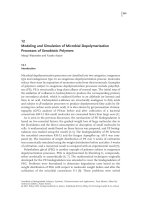
Figure 9.6. Top to bottom and left to right, the progressive movement of rays
making up a beam (L = 0.325 and ˆn = 10). The lengths of the vectors indicate the
irradiance (Zohdi [219]).
05 book
2007/5/15
page 116
✐
✐
✐
✐
✐
✐
✐
✐
116 Chapter 9. Simple optical scattering methods for particulate media

def
= (L, ˆn), an ensemble averaging procedure is applied whereby the performances of a
series of different random starting scattering configurations are averaged until the (ensem-

ble) average converges, i.e., until the following condition is met:





1
M + 1
M+1

i=1

(i)
(
I
) −
1
M
M

i=1

(i)
(
I
)






≤ TOL





1
M + 1
M+1

i=1

(i)
(
I
)





,
where index i indicates a different starting random configuration (i = 1, 2, ,M) that
has been generated and M indicates the total number of configurations tested. Similar ideas
have been applied to determine responses of other types of randomly dispersed particulate
media in Zohdi [208]–[213]. Typically, between 10 and 20 ensemble sample averages need
to be performed for  to stabilize.
Remark. As before, in order to generate the random particle positions, the classical
random sequential addition algorithm was used to place nonoverlapping particles into the

domain of interest (Widom [200]). This algorithm was adequate for the volume fraction
ranges of interest (under 30%).
Remark. It is important to recognize that one can describe the aggregate ray behavior
described in this work in a more detailed manner via higher moment distributions of the
individual ray fronts and their velocities. For example, consider any quantity, Q, with a
distribution of values (Q
i
,i = 1, 2, ,N
r
= rays) about an arbitrary reference value,
denoted Q

, as follows:
M
Q
i
−Q

p
def
=

N
r
i=1
(Q
i
− Q

)

p
N
r
def
= (Q
i
− Q

)
p
,
(9.40)
where

N
r
i=1
(·)
N
r
def
= (·) (9.41)
and A
def
= Q
i
. The various moments characterize the distribution, for example, (I) M
Q
i
−A

1
measures the first deviation from the average, which equals zero, (II) M
Q
i
−0
1
is the average,
(III) M
Q
i
−A
2
is the standard deviation, (IV) M
Q
i
−A
3
is the skewness, and (V) M
Q
i
−A
4
is the
kurtosis. The higher moments, such as the skewness, measure the bias, or asymmetry, of the
distribution of data, while the kurtosis measures the degree of peakedness of the distribution
of data around the average. The skewness is zero for symmetric data. The specification of
these higher moments can be input into a cost function in exactly the same manner as the
average. This was not incorporated in the present work.
9.3.2 Results for spherical scatterers
Figure 9.7 indicates that, for a given value of ˆn,  depends in a mildly nonlinear manner on

the particulate length scale (L). Furthermore, there is a distinct minimum value of L to just
block all of the incoming rays. Atypicalvisualization for a simulation of the ray propagation
is given in Figure 9.6. Clearly, the point where  = 0, for each curve, represents the length
scale that is just large enough to allow no rays to penetrate the system. For a given relative
refractive index ratio, length scales larger than a critical value force more of the rays to
be scattered backward. Table 9.1 indicates the estimated values for the length scale and
05 book
2007/5/15
page 117
✐
✐
✐
✐
✐
✐
✐
✐
9.3. Multiple scatterers 117
-0.2
-0.15
-0.1
-0.05
0
0.05
0.1
0.15
0.2
0.24 0.26 0.28 0.3 0.32 0.34 0.36 0.38
PI
LENGTH SCALE

N-HAT=2
N-HAT=4
N-HAT=10
N-HAT=100
Figure 9.7. The variation of  as a function of L (Zohdi [218]).
Table 9.1. The estimated volume fractions needed for no complete penetration of
incident electromagnetic energy,  = 0.
ˆn L v
p
=
4πL
3
3
2 0.4200
0.3107
4
0.3430 0.1692
10 0.3125 0.1278
100 0.2850 0.0969
the corresponding volume fraction needed to achieve no penetration of the electromagnetic
rays, i.e.,  = 0. Clearly, at some point there are diminishing returns to increasing the
volume fraction for a fixed refractive index ratio (ˆn). A least-squares curve fit indicates the
following relationships between L and ˆn, as well as between the volume fraction v
p
and ˆn,
for  = 0 to be achieved:
L = 0.4090ˆn
−0.0867
or v
p

= 0.2869ˆn
−0.2607
. (9.42)
Qualitatively speaking, these results suggest the intuitive trend that if one has more reflective
particles, one needs fewer of them to block (in a vectorially averaged sense) incoming rays,
and vice versa.
To further understand this behavior, consider a single reflecting scatterer, with incident
rays as shown in Figure 9.8. All rays at an incident angle between
π
2
and
π
4
are reflected with
some positive y-component, i.e., “backward” (back scatter). However, between
π
4
and 0,
the rays are scattered with a negative y-component, i.e., forward. Since the reflectance is the
ratio of the amount of reflected energy (irradiance) to the incident energy, it is appropriate
to consider the integrated reflectance over a quarter of a single scatterer, which indicates
the total fraction of the irradiance reflected:
I
def
=
1
π
2

π

2
0
Rdθ, (9.43)
whose variation with ˆn is shown in Figure 9.9. In the range tested of 2 ≤ˆn ≤ 100, the
05 book
2007/5/15
page 118
✐
✐
✐
✐
✐
✐
✐
✐
118 Chapter 9. Simple optical scattering methods for particulate media
Θ
Θ
Θ
y
incoming
reflected
x
0.2
0.3
0.4
0.5
0.6
0.7
0.8

0.9
1
0 200 400 600 800 1000 1200
INTEGRATED REFLECTANCE
N-hat
Figure 9.8. Left, a single scatterer. Right, the integrated reflectance (I) over a
quarter of a single scatterer, which indicates the total fraction of the irradiance reflected
(Zohdi [219]).
-0.05
0
0.05
0.1
0.15
0.2
0.25
0.3
0.35
0.24 0.26 0.28 0.3 0.32 0.34 0.36 0.38
PI
LENGTH SCALE
N-HAT=2
N-HAT=4
N-HAT=10
N-HAT=100
Figure9.9. (Oblate) Ellipsoids of aspect ratio 4:1: The variation of  as afunction
of L. The volume fraction is given by v
p
=
πL
3

4
(Zohdi [219]).
amount of energy reflected is a mildly nonlinear (quasi-linear) function of ˆn for a single
scatterer, and thus it is not surprising that it is the same for an aggregate.
9.3.3 Shape effects: Ellipsoidal geometries
One can consider a more detailed description of the scatterers, where we characterize the
shape of the particles by the equation for an ellipsoid:
62
F
def
=

x − x
o
r
1

2
+

y − y
o
r
2

2
+

z − z
o

r
3

2
= 1.
(9.44)
62
The outward surface normals needed during the scattering process are relatively easy to characterize by
writing n =
∇F
||∇F ||
. The orientation of the particles, usually random, can be controlled via rotational coordinate
transformations.
05 book
2007/5/15
page 119
✐
✐
✐
✐
✐
✐
✐
✐
9.4. Discussion 119
As an example, consider oblate spheroids with an aspect ratio of AR =
r
1
r
2

=
r
1
r
3
= 0.25. As
shown in Figure 9.9, the intuitive increase in volume fraction leads to an increase in overall
reflectivity. The reason for this is that the volume fractions are so low, due to the fact that
the particles are oblate, that the point of diminishing returns ( = 0) is not met with the
same length scale range as tested for the spheres. The volume fraction, for oblate spheroids
given by AR ≤ 1, is
v
p
=
4ARπL
3
3
, (9.45)
where the largest radius (r
2
or r
3
) is used to calculate L. The volume fraction of a system
containing oblate ellipsoidal particles, for example, with AR = 0.25, is much lower (one-
sixteenth) than that of a system containing spheres with the same length scale parameter
L. As seen in Figure 9.9, at relatively high volume fractions (L = 0.375), with the highest
(idealized, mirror-like) reflectivity tested (ˆn = 100), the effect of “diminishing returns”
begins, as it had for the spherical case. Clearly, it appears to be an effect that requires
relatively high volume fractions to block the incoming rays, and consequently the effects
of shape appear minimal for overall scattering.

Remark. Recently, a computationalframeworkto rapidlysimulatethe light-scattering
response of multiple red blood cells (RBCs), based upon ray-tracing, was developed in Zo-
hdi and Kuypers [223]. Because the wavelength of visible light (roughly 3.8 × 10
−7
m ≤
λ ≤ 7.8×10
−7
m) is approximately at least an order of magnitude smaller than the diameter
of a typical RBC scatterer (d ≈ 8 ×10
−6
m), geometric ray-tracing theory is applicable and
can be used to quickly ascertain the amount of optical energy, characterized by the Poynting
vector, that is reflected and absorbed by multiple RBCs. Three-dimensional examples were
given to illustrate the approach, and the results compared quite closely to experiments on
blood samples conducted at the Children’s Hospital Oakland Research Institute (CHORI).
See Appendix B for more details.
9.4 Discussion
For the disordered particulate systems considered, as the volume fraction of the scatter-
ing particles increases, as one would expect, less incident energy penetrates the aggregate
particulate system. Above this critical volume fraction, more rays are scattered backward.
However, the volume fraction at which the point of no penetration occurs depends in a quasi-
linear fashion upon the ratio oftherefractiveindicesofthe particle and surrounding medium.
The similarity of electromagnetic scattering to acoustical scattering, governing sound
disturbances that travels in inviscid media, is notable. Of course, the scales at which ray
theory can be applied are much different because sound wavelengths are much larger than
the wavelengths of light. The reflection of a plane harmonic pressure wave energy at an
interface is given by
63
R =


P
r
P
i

2
=

ˆ
A cos θ
i
− cos θ
t
ˆ
A cos θ
i
+ cos θ
t

2
, (9.46)
where P
i
is the incident pressure ray, P
r
is the reflected pressure ray,
ˆ
A
def
=

ρ
t
c
t
ρ
i
c
i
, ρ
t
is
the medium the ray encounters (transmitted), c
t
is the corresponding sound speed in that
63
This relation is derived in Appendix B.
05 book
2007/5/15
page 120
✐
✐
✐
✐
✐
✐
✐
✐
120 Chapter 9. Simple optical scattering methods for particulate media
-0.04
-0.02

0
0.02
0.04
0.06
0.08
0.1
0.12
0.14
0.16
0.24 0.26 0.28 0.3 0.32 0.34 0.36 0.38
PI
LENGTH SCALE
C-HAT=0.5
C-HAT=0.25
C-HAT=0.1
C-HAT=0.01
Figure 9.10. Results for acoustical scattering (ˆc = 1/˜c) (Zohdi [219]).
medium, ρ
i
is the medium in which the ray was traveling (incident), and c
i
is the correspond-
ing sound speed in that medium. Clearly, the analysis of the aggregates can be performed for
acoustical scattering in essentially the same way as for the optical problem. For example,
for the same model problem as for the optical scenario (400 rays, 1000 scatterers), however,
with the geometry and velocity appropriately scaled,
64
the results are shown in Figure 9.10
for varying ˆc =
c

t
c
i
= 1/ ˜c. The results for the acoustical analogy are quite similar to those
for optics. See Appendix B for more details.
As mentioned earlier, for most materials the magnetic permeability is virtually the
same, with exceptions being concentrated magnetite, pyrrhotite, and titanomagnetite (see
Telford et al. [192] and Nye [153]). Clearly, with many new industrial materials being
developed, possibly having nonstandard magnetic permeabilities ( ˆµ = 1), such effects may
become more important to consider. Generally, from studying Equation (9.36), as ˆµ →∞,
R → 1. In other words, as the relative magnetic permeability increases, the reflectance
increases. More remarks are given in Appendix B.
Obviously, when more microstructural features are considered, for example, topolog-
ical and thermal variables, parameter studies become quite involved. In order to eliminate a
trial and error approach to determining the characteristics of the types of particles that would
be needed to achieve acertain level of scattering, in Zohdi [218] an automated computational
inverse solution technique has recently been developed to ascertain particle combinations
that deliver prespecified electromagnetic scattering, thermal responses, and radiative (in-
frared) emission, employing genetic algorithms in combination with implicit staggering so-
lution schemes, based upon approaches found in Zohdi [212]–[218]. This is discussed next.
9.5 Thermal coupling
The characterization of particulate systems, flowing or static, must usually be conducted in
a nonevasive manner. Thus, experimentally speaking, light-scattering behavior can be a key
64
Typical sound wavelengths are in the range of 0.01 m ≤ λ ≤ 30 m, with wavespeeds in the range of 300 m/s
≤ c ≤ 1500 m/s, thus leading to wavelengths, f = c/λ, with ranges on the order of 10 1/s ≤ f ≤ 150000 1/s.
Therefore, the scatterers must be much larger than scatterers in applications involving ray-tracing in optics.
05 book
2007/5/15
page 121

✐
✐
✐
✐
✐
✐
✐
✐
9.5. Thermal coupling 121
indicator of the character of the flow. Experimentally speaking, thermal behavior can be a
key indicator of the dynamical character of particulate flows. For example, in Chung et al.
[45] and Shin et al. [177], techniques for measuring flow characteristics based upon infrared
thermal velocimetry (ITV) in fluidic microelectromechanical systems (MEMS) have been
developed. In such approaches, infrared lasers are used to generate a short heating pulse
in a flowing liquid, and an infrared camera records the radiative images from the heated
flowing liquid. The flow properties are obtained from consecutive radiative images. This
approach is robust enough to measure particulate flows as well. In such approaches, a
heater generates a short thermal pulse, and a thermal sensor detects the arrival downstream.
This motivates the investigation of the coupling between optical scattering (electromagnetic
energy propagation) and thermal coupling effects for particulate suspensions.
As before, it is assumed that the scattering particles are small enough to consider
that the temperature fields are uniform in the particles.
65
We consider an energy balance,
governing the interconversions of mechanical, thermal, and chemical energy in a system,
dictated by the first law of thermodynamics. Accordingly, we require the time rate of change
of the sum of the kinetic energy (K) and stored energy (S) to be equal to the sum of the
work rate (power, P) and the net heat supplied (H):
d
dt

(K + S) = P +H, (9.47)
where the stored energy comprises a thermal part, S(t) = mCθ(t ), where C is the heat
capacity per unit mass, and, consistent with our assumptions that the particles deform
negligibly during the process, a negligible mechanical stored energy portion. The kinetic
energy is K(t) =
1
2
mv(t) ·v(t). The mechanical power term is due to the total forces (
tot
)
acting on a particle, namely,
P =
dW
dt
= 
tot
· v. (9.48)
Also, because
dK
dt
= m
˙
v ·v(t), and we have a balance of momentum m
˙
v ·v = 
tot
·v, thus
dK
dt
=

dW
dt
= P, leading to
dS
dt
= H. The primary source of heat is due to the incident rays.
The energy input from the reflection of a ray is defined as
H
rays
def
=

t+t
t
H
rays
dt ≈ (I
i
− I
r
)a
r
t = (1 −R)I
i
a
r
t. (9.49)
After an incident ray is reflected, it is assumed that a process of heat transfer occurs (Fig-
ure 9.11). It is assumed that the temperature fields are uniform within the particles; thus,
conduction within the particles is negligible. We remark that the validity of using a lumped

thermal model, i.e., ignoring temperature gradients and assuming a uniform temperature
within a particle, is dictated by the magnitude of the Biot number. A small Biot number
indicates that such an approximation is reasonable. The Biot number for spheres scales with
the ratio of particle volume (V ) to particle surface area (a
s
),
V
a
s
=
b
3
, which indicates that a
uniform temperature distribution is appropriate, since the particles, by definition, are small.
65
Thus, the gradient of the temperature within the particle is zero, i.e., ∇θ = 0. Therefore, a Fourier-type law
for the heat flux will register a zero value, q =−K ·∇θ = 0. Furthermore, we assume that the space between the
particles, i.e., the “ether,” plays no role in the heat transfer process.
05 book
2007/5/15
page 122
✐
✐
✐
✐
✐
✐
✐
✐
122 Chapter 9. Simple optical scattering methods for particulate media

CONTROL
VOLUME
i
I
I
r
Figure 9.11. Control volume for heat transfer (Zohdi [218]).
The first law reads
d(K + S)
dt
= m
˙
v ·v +mC
˙
θ = 
tot
· v

 
mechanical power
− h
c
a
s
(θ − θ
o
)

 
convective heating

−Ba
s
ε(θ
4
− θ
4
s
)

 
thermal radiation
+H
rays

sources
,
(9.50)
where θ
o
is the temperature of the ambient gas; θ
s
is the temperature of the far-field surface
(for example, a container surrounding the flow) with which radiative exchange is made;
B = 5.67 × 10
−8
W
m
2
·K
is the Stefan–Boltzmann constant; 0 ≤ ε ≤ 1 is the emissivity,

which indicates how efficiently the surface radiates energy compared to a black-body (an
ideal emitter); 0 ≤ h
c
is the heating due to convection (Newton’s law of cooling) into the
dilute gas; and a
s
is the surface area of a particle. It is assumed that the thermal radiation
exchange between the particles is negligible. For the applications considered here, typically,
h
c
is quite small and plays a small role in the heat transfer processes. From a balance of
momentum we have m
˙
v ·v = 
tot
· v and Equation (9.49) becomes
mC
˙
θ =−h
c
a
s
(θ − θ
o
) − Ba
s
ε(θ
4
− θ
4

s
) + H
rays
.
(9.51)
Therefore, after temporal integration with a finite difference time step of t, we have
θ(t +t) =
1
mC + h
c
a
s
t

mCθ(t) −tBa
s
ε

θ
4
(t +t) − θ
4
s

+th
c
a
s
θ
o

+H
rays

.
(9.52)
This implicit nonlinear equation for θ, for each particle, is added into the ray-tracing
algorithm in the next section.
9.6 Solution procedure
We now develop a staggering scheme by extending an approach found in Zohdi [208]–
[210], [212], and [213]. After time discretization of the stored energy term in the equations
of thermal equilibrium for a particle,
mC
˙
θ
L+1
i
≈ mC
θ
L+1
i
− θ
L
i
t
, (9.53)
05 book
2007/5/15
page 123
✐
✐

✐
✐
✐
✐
✐
✐
9.6. Solution procedure 123
() COMPUTE RAY ORIENTATIONS AFTER REFLECTION (FRESNEL RELATIONS);
COMPUTE ABSORPTION CONTRIBUTIONS TO THE PARTICLES: H
rays
;
COMPUTE PARTICLE TEMP. (RECURSIVELY, K = 1, 2, UNTIL CONVERGENCE):
θ
L+1,K
=
1
mC +h
c
a
s
t

mCθ
L
− tBa
s
ε

(θ
L+1,K−1

)
4
− θ
4
s

+ th
c
a
s
θ
o
+ H
rays

;
INCREMENT ALL RAY POSITIONS: r
i
(t + t) = r
i
(t) + tv
i
(t);
GO TO () AND REPEAT (t = t +t).
Algorithm 9.2
where, for brevity, we write θ
i
L+1
def
= θ

i
(t +t), θ
i
L
def
= θ
i
(t), etc., we arrive at the abstract
form, for the entire system, of A(θ
L+1
i
) = F. It is convenient to write
A(θ
L+1
i
) − F = G(θ
L+1
i
) − θ
L+1
i
+ R = 0, (9.54)
where R is a remainder term that does not depend on the solution, i.e., R = R(θ
L+1
i
).A
straightforward iterative scheme can be written as
θ
L+1,K
i

= G(θ
L+1,K−1
i
) + R, (9.55)
where K = 1, 2, 3, is the index of iteration within time step L +1. The convergence of
such a scheme depends on the behavior of G. Namely, a sufficient condition for convergence
is that G be a contraction mapping for all θ
L+1,K
i
, K = 1, 2, 3, In order to investigate
this further, we define the error as θ
L+1,K
= θ
L+1,K
i
− θ
L+1
i
. A necessary restriction
for convergence is iterative self-consistency, i.e., the exact solution must be represented
by the scheme G(θ
L+1
i
) + R = θ
L+1
i
. Enforcing this restriction, a sufficient condition for
convergence is the existence of a contraction mapping of the form
||θ
L+1,K

||=||θ
L+1,K
i
−θ
L+1
i
||=||G(θ
L+1,K−1
i
) −G(θ
L+1
i
)||≤η
L+1,K
||θ
L+1,K−1
i
−θ
L+1
i
||,
(9.56)
where, if η
L+1,K
< 1 for eachiteration K, thenθ
L+1,K
→ 0 for anyarbitrary starting value
θ
L+1,K=0
i

as K →∞. The type of contraction condition discussed is sufficient, but not
necessary, for convergence. Typically, the time step sizes for ray-tracing are far smaller than
needed; thus, the approach converges quickly. More specifically, G’s behavior is controlled
by
tBa
s
ε
mC+h
c
a
s
t
, which is quite small. Thus, a fixed-point iterative scheme, such as the one
introduced, converges rapidly. This iterative procedure is embedded into the overall ray-
tracing scheme. For the overall algorithm (starting at t = 0 and ending at t = T ), see
Algorithm 9.2.
In order to capture all of the internal reflections that occur when rays enter the par-
ticulate systems, the time step size t is dictated by the size of the particles. A somewhat
ad hoc approach is to scale the time step size according to t = ξb, where b is the radius
of the particles and typically 0.05 ≤ ξ ≤ 0.1.
05 book
2007/5/15
page 124
✐
✐
✐
✐
✐
✐
✐

✐
124 Chapter 9. Simple optical scattering methods for particulate media
9.7 Inverse problems/parameter identification
An important aspect of any model is the inverse problem of identifying parameters that force
the system behavior to match a target response and may stem from an experimental obser-
vation or a design specification. In the ideal case, one would like to determine combinations
of scattering parameters that produce certain aggregate effects, via numerical simulations,
in order to minimize time-consuming laboratory tests. The primary quantity of interest in
this work is the percentage of lost irradiance by a beam in a selected direction over the time
interval of (0,T). As in the previous examples, this is characterized by the inner product
of the Poynting vector and a selected direction (d):
Z(0,T)
def
=

N
r
i=1
(S(t = 0) − S(t = T))· d

N
r
i=1
S
i
(t = 0) · d
, (9.57)
where Z can be considered the amount of energy “blocked” (in a vectorially averaged sense)
from propagating in the d direction. Now consider a cost function comparing the loss to
the specified blocked amount:


def
=




Z(0,T)− Z
∗
Z
∗




, (9.58)
where the total simulation time is T and where Z
∗
is a target blocked value. One can
augment this by also monitoring the average temperature of the scattering particles during
the time interval,
(0,T)
def
=
1
N
p
T

T

0
N
p

i=1
θ
i
(t) dt, (9.59)
as well as the average emitted thermal radiation of the scatterers during the time interval,
(0,T)
def
=
1
N
p
T

T
0
N
p

i=1
Ba
si
ε
i
(θ
4
i

(t) − θ
4
s
)dt, (9.60)
to yield the composite cost function
(w
1
,w
2
,w
3
)
def
=
1

3
j=1
w
j

w
1




Z(0,T)− Z
∗
Z

∗




+ w
2




(0,T)−
∗

∗




+ w
3




(0,T)− 
∗

∗






,
(9.61)
where 
∗
and 
∗
are specified values. Typically, for the class of problems considered in this
work, formulations such as in Equation (9.61) depend in a nonconvex and nondifferentiable
manner on the system parameters. With respect to the minimization of Equation (9.61), clas-
sical gradient-based deterministic optimization techniques are not robust due to difficulties
with objective function nonconvexity and nondifferentiability. Classical gradient-based al-
gorithms are likely to converge only toward a local minimum of the objective function if an
accurate initial guess for the global minimum is not provided. Also, usually it is extremely
difficult to construct an initial guess that lies within the (global) convergence radius of a
05 book
2007/5/15
page 125
✐
✐
✐
✐
✐
✐
✐
✐
9.8. Parametrization and a genetic algorithm 125

gradient-based method. These difficulties can be circumvented by using a certain class
of nonderivative search methods, i.e., genetic algorithms, before applying gradient-based
schemes. Genetic algorithms are search methods based on the principles ofnatural selection,
employing concepts of species evolution such as reproduction, mutation, and crossover. Im-
plementation typically involves a randomly generated population of fixed-length elemental
strings, “genetic information,” each of which represents a specific choice of system param-
eters. The population of individuals undergoes “mating sequences” and other biologically
inspired events in order to find promising regions of the search space. There are a variety of
such methods, employing concepts of species evolution such as reproduction, mutation, and
crossover. Such methods primarily stem from the work of John Holland (Holland [94]). For
reviews of such methods, see, for example, Goldberg [77], Davis [50], Onwubiko [155],
Kennedy and Eberhart [120], Lagaros et al. [129], Papadrakakis et al. [156]–[159] and
Goldberg and Deb [78].
Remark. To compute thefitness of a parameter set, onemust go through the procedure
in Algorithm 9.2, requiring a full-scale simulation. It is important to scale the system vari-
ables, for example, to be positive numbers and of comparable magnitude, in order to avoid
dealing with large variations in the parameter vector components. Typically, for particulate
flows with a finite number of particles, there will be slight variations in the performance for
different random starting configurations. In order to stabilize the objective function’s value
with respect to the randomness of the flow starting configuration, for a given parameter
selection (), a regularization procedure is applied within the genetic algorithm, whereby
the performances of a series of different random starting configurations are averaged until
the (ensemble) average converges, i.e., until the following condition is met:





1
Z +1

Z+1

i=1

(i)
(
I
) −
1
Z
Z

i=1

(i)
(
I
)





≤ TOL





1

Z +1
Z+1

i=1

(i)
(
I
)





,
where index i indicates a different starting random configuration (i = 1, 2, ,Z) that
has been generated and Z indicates the total number of configurations tested. In order to
implement this in the genetic algorithm, in Step 2, one simply replaces compute with ensem-
ble compute, which requires a further inner loop to test the performance of multiple starting
configurations. Similar ideas have been applied to other types of randomly dispersed par-
ticulate media in Zohdi [208]–[213]. Clearly, such a procedure is not necessary when the
scatterers are periodically arranged.
Remark. As before, the classical random sequential addition algorithm was used to
place nonoverlapping particles into the domain of interest (Widom [200]). This algorithm
was adequate for the volume fraction ranges of interest (under 30%).
9.8 Parametrization and a genetic algorithm
We considered a group of N
p
randomly positioned particles, of equal size, in a cube of
normalized dimensions, D × D × D, with D normalized to unity. The particle size

and volume fraction were determined by a particle/sample size ratio, which was defined
via a subvolume size V
def
=
D×D×D
N
p
, where N
p
was the number of particles in the entire
cube (Figure 9.12). The ratio between the radius (b) and the subvolume was denoted by
05 book
2007/5/15
page 126
✐
✐
✐
✐
✐
✐
✐
✐
126 Chapter 9. Simple optical scattering methods for particulate media
)(
1/3
b
TOTAL SAMPLE DOMAIN
V/N
Figure 9.12. Definition of a particle length scale (Zohdi [218]).
0

0.2
0.4
0.6
0.8
1
1.2
1.4
1.6
1.8
2
0 5 10 15 20
FITNESS
GENERATION
Figure 9.13. The best parameter set’s objective function values for successive
generations. Note: The first data point in the optimization corresponds to the objective
function’svalue formean parameter values ofupper and lowerbounds of the searchintervals
(Zohdi [218]).
L
def
=
b
V
1
3
. The volume fraction occupied by the particles was v
p
def
=
4πL
3

3
. Thus, the total
volume occupied by the particles, denoted by ν, can be written as ν = v
p
N
p
V . We used
N
p
= 1000 particles and N
r
= 400 rays, arranged in a square 20×20 pattern (Figure 9.14).
This system provided stable results, i.e., increasing the number of rays and/or the number
of particles beyond these levels resulted in negligibly different overall system responses.
The free parameters in the inverse problem were as follows:
• The particle length scale was 0 < L ≤ 0.35.
• The relative refractive index ratio was 1 < ˆn ≤ 10.
• The particle emissivity was 0 ≤ ε ≤ 1.
• The particle density, combined with the heat capacity, was (ρC)
−
≤ (ρC) ≤ (ρC)
+
,
where mC = ρ
4
3
πb
3
C. C was held fixed at C = 10
3

N · m/
◦
K and 10
3
kg/m
3
=
ρ
−
≤ ρ ≤ ρ
+
= 2 ×10
3
kg/m
3
.
05 book
2007/5/15
page 127
✐
✐
✐
✐
✐
✐
✐
✐
9.8. Parametrization and a genetic algorithm 127
518.809
504.222

489.635
475.048
460.46
445.873
431.286
416.698
402.111
387.524
372.936
358.349
343.762
329.175
314.587
518.809
504.222
489.635
475.048
460.46
445.873
431.286
416.698
402.111
387.524
372.936
358.349
343.762
329.175
314.587
518.809
504.222

489.635
475.048
460.46
445.873
431.286
416.698
402.111
387.524
372.936
358.349
343.762
329.175
314.587
518.809
504.222
489.635
475.048
460.46
445.873
431.286
416.698
402.111
387.524
372.936
358.349
343.762
329.175
314.587
Figure 9.14. Top to bottom and left to right, the progressive movement of rays
making up a beam (for the best inverse parameter set vector (Table 9.2)). The colors of the

particles indicate their temperature and the lengths of the vectors indicate the irradiance
magnitude (Zohdi [218]).
Thus, explicitly, the genetic string comprised the following parameters:
 = (L,ρC,,ˆn). (9.62)
Other simulation parameters of importance are as follows:
• The dimensions of the sample were 10
−3
m ×10
−3
m ×10
−3
m.
• The time scale was set to
3×10
−3
m
c
, where c = 3 × 10
8
m/s is the speed of light.
• The initial velocity vector for all initially collinear rays making up the beam was
v = (c, 0, 0).
• The irradiance beam parameter was set to I = 10
18
N ·m/(m
2
·s), where the irradiance
for each ray was calculated as I
ray
(t = 0)a

r
def
= Ia
b
/N
r
, where N
r
= 20 ×20 = 400
05 book
2007/5/15
page 128
✐
✐
✐
✐
✐
✐
✐
✐
128 Chapter 9. Simple optical scattering methods for particulate media
Table 9.2. The optimal scattering parameters and the top six fitnesses with w
1
=
w
2
= w
3
= 1.
Rank L

ˆn ε ρ × 10
−3
kg/m
3

1 0.21480 5.82056 0.53687 0.15078 0.04968310
2
0.21481 5.91242 0.53741 0.15152 0.05126406
3 0.21482 5.89121 0.53637 0.15152 0.05166210
4
0.21482 5.83350 0.53636 0.15150 0.05232877
5 0.21477 6.23032 0.53748 0.16034 0.05236720
6 0.21481 5.81637 0.53672 0.15008 0.05260397
is the number of rays in the beam and a
b
= 10
−3
m ×10
−3
m = 10
−6
m
2
is the
cross-sectional area of the beam.
• The first two objectives were Z
∗
= 0.75 and 
∗
= 400

◦
K. A convenient way to
parametrize 
∗
is to write it as a percentage of the incident energy per unit time of
the entire beam, K
∗
I
ray
(t = 0) × N
r
, where 0 ≤ K
∗
≤ 1. A value of K
∗
= 10
−18
was chosen.
The number of genetic strings in the population was set to 20, for 20 generations,
allowing 6 offspring of the top 6 parents, along with their parents, to proceed to the next
generation. Therefore, after each generation, 8 entirely new genetic strings were intro-
duced. Every 10 generations, the search was rescaled around the best parameter set, and
the search restarted. Table 9.2 and Figure 9.13 depict the results. A total of 286 parameter
selections were tested. The behavior of the best parameter selection’s response is shown in
Figures 9.14 and 9.15. The total number of strings tested was 3651, thus requiring an aver-
age of 12.765 strings per parameter selection for the ensemble averaging stabilization. After
approximately 6 generations, the procedure stabilized. We again remark that gradient-based
methods are sometimes useful for postprocessing solutions found with a genetic algorithm,
if the objective function is sufficiently smooth in that region of the parameter space. This
was not done in this work; however, the reader can consult the texts of Luenberger [142]

and Gill et al. [76], or the survey in Papadrakakis et al. [160].
9.9 Summary
The presented work developed a ray-tracing algorithm that was combined with a stochastic
genetic algorithm in order to treat coupled inverse optical scattering formulations, where
physical parameters, such as particulate volume fractions, refractive indices, and thermal
constants, were sought so that the overall response of a sample of randomly distributed par-
ticles, suspended in an ambient medium, would match desired coupled scattering, thermal,
and infrared responses. Large-scale numerical simulations were presented to illustrate the
overall procedure and to investigate aggregate ray dynamics corresponding to the flow of
electromagnetic energy and the conversion of the absorbed energy into heat and infrared
radiation through disordered particulate systems.
Such design methodologies may be helpful in designing optical coating materials
comprising randomly dispersed particles suspended in a binding matrix. The matrix usually
05 book
2007/5/15
page 129
✐
✐
✐
✐
✐
✐
✐
✐
9.9. Summary 129
518.809
504.222
489.635
475.048
460.46

445.873
431.286
416.698
402.111
387.524
372.936
358.349
343.762
329.175
314.587
518.809
504.222
489.635
475.048
460.46
445.873
431.286
416.698
402.111
387.524
372.936
358.349
343.762
329.175
314.587
518.809
504.222
489.635
475.048
460.46

445.873
431.286
416.698
402.111
387.524
372.936
358.349
343.762
329.175
314.587
518.809
504.222
489.635
475.048
460.46
445.873
431.286
416.698
402.111
387.524
372.936
358.349
343.762
329.175
314.587
Figure9.15. Continuing Figure9.14, top to bottomand leftto right, the progressive
movement of rays making up a beam (for the best inverse parameter set vector (Table 9.2)).
The colors of the particles indicate their temperature and the lengths of the vectors indicate
the irradiance magnitude (Zohdi [218]).
has good adhesive and mechanical properties, while the particles are used as scattering

units. Such coatings are relatively inexpensive to fabricate. The overall optical properties
of such materials can be tailored by adjusting the volume fraction and refractive index of
the particulate additives.
Accordingly, we can consider a more detailed description of the scatterers, where we
characterize the shape of the particles by a generalized ellipsoidal equation:
66
F
def
=

|x − x
o
|
r
1

s
1
+

|y − y
o
|
r
2

s
2
+


|z − z
o
|
r
3

s
3
= 1,
(9.63)
where the s’s are exponents. The orientation of the particles, usually random, can be
controlled via rotational coordinate transformations. Values of s<1 produce nonconvex
66
The outward surface normals, n, needed during the scattering calculations, are relatively easy to characterize
by writing n =
∇F
||∇F ||
.
05 book
2007/5/15
page 130
✐
✐
✐
✐
✐
✐
✐
✐
130 Chapter 9. Simple optical scattering methods for particulate media

-0.0008
-0.0006
-0.0004
-0.0002
0
0.0002
0.0004
0.0006
0 0.002 0.004 0.006 0.008 0.01 0.012 0.014
AVERAGE POSITION (M)
TIME (NANO-SEC)
RX
RY
RZ
-0.2
0
0.2
0.4
0.6
0.8
1
1.2
0 0.002 0.004 0.006 0.008 0.01 0.012 0.014
NORMALIZED VELOCITY
TIME (NANO-SEC)
<Vx>/c
<Vy>/c
<Vz>/c
||V||/c
Figure 9.16. Top, the components of the average position over time for the best

parameter set. Bottom, the components of the average ray velocity and the Euclidean norm
over time for the best parameter set. The normalized quantity ||v||/c = 1 serves as a type
of computational “error check” (Zohdi [218]).
shapes, while s>2 values produce “block-like” shapes (three inverse parameters). Further-
more, we can introduce the particulate aspect ratio, defined by AR
def
=
r
1
r
2
=
r
1
r
3
, where
r
2
= r
3
, AR > 1 for prolate geometries, and AR < 1 for oblate shapes (one variable).
Therefore, including the variables introduced before, in the most general case we have a
total of nine variables,  = (L,ρC,,ˆn, ˆµ, s
1
,s
2
,s
3
,AR). We remark that if the particles’

orientations are assumed aligned, then three more (angular orientation) parameters can
be introduced, (θ
1
,θ
2
,θ
3
). In fact, suspensions can become aligned, for example, along
electrical field lines induced by external sources, or due to flow conditions. Thus, the search
space grows to 12 parameters,
67
 = (L,ρC,,ˆn, ˆµ, s
1
,s
2
,s
3
,AR,θ
1
,θ
2
,θ
3
).
67
It is important to note that the control of the particle properties, volume fractions, orientations, etc., can be
used to design hybrid thin films composed of particulate additives in a matrix binder.
05 book
2007/5/15
page 131

✐
✐
✐
✐
✐
✐
✐
✐
9.9. Summary 131
-0.2
0
0.2
0.4
0.6
0.8
1
0 0.002 0.004 0.006 0.008 0.01 0.012 0.014
NORMALIZED IRRADIANCE
TIME (NANO-SEC)
Ix/||I(0)||
Iy/||I(0)||
Iz/||I(0)||
||I(t)||/||I(0)||
300
310
320
330
340
350
360

370
380
390
0 0.002 0.004 0.006 0.008 0.01 0.012 0.014
AVERAGE PARTICLE TEMPERATURE (K)
TIME (NANO-SEC)
TEMP
Figure 9.17. Top, the components of the average ray irradiance and the Euclidean
norm over time for the best parameter set. Bottom, the average temperature of the scatterers
over time for the best parameter set (Zohdi [218]).
0
2e-07
4e-07
6e-07
8e-07
1e-06
1.2e-06
1.4e-06
0 0.002 0.004 0.006 0.008 0.01 0.012 0.014
TOTAL EMITTED THERMAL RADIATION (N-M/SEC)
TIME (NANO-SEC)
RAD
Figure 9.18. The average thermal radiation of the scatterers over time for the best
parameter set (Zohdi [218]).
05 book
2007/5/15
page 132
✐
✐
✐

✐
✐
✐
✐
✐
132 Chapter 9. Simple optical scattering methods for particulate media
Finally, in addition to a more detailed characterization of the particle geometry, in
some cases transparent particle materials, accounting for refractive and dispersive rays
traveling through scatterers, can be important. Recall that the dispersion of a light ray is
how, for example, white light, which is a mixture of all wavelengths of visible light, can be
decomposed into its constituent wavelengths or colors when it passes from one medium into
another. This phenomenon occurs because the index of refraction of a transparent medium
is greater for light of shorter wavelengths. Thus, whenever light is refracted in passing
from one medium to the next, the violet and blue light of shorter wavelengths is bent more
than the orange and red light of longer wavelengths.
68
Thus, dispersive effects introduce
a new level of complexity, primarily because of the refraction of different wavelengths of
light, leading to a dramatic growth in the number of rays of varying intensities and color
(wavelength). The inclusion of these effects is currently under investigation by the author.
68
This is how a rainbow is formed.
05 book
2007/5/15
page 133
✐
✐
✐
✐
✐

✐
✐
✐
Chapter 10
Closing remarks
This monograph provided a basic introduction to the subject of particulate flows. Clearly, a
comprehensive survey of all the possible modeling and computational techniques cannot be
undertaken in awork of this size. However, an extensivelist of references hasbeen provided.
In particular, we note that a survey of fast computational methods, specifically efficient
contact search techniques for the treatment of densely packed granular or particulate media,
in the absence of near-field forces, can be found in the recent work of Pöschel and Schwager
[167]. However, while such techniques are outside the scope of the present work, they
are relatively easy to implement and are highly recommended to attain high-performance
simulations for large numbers of particles, in particular when they are irregularly shaped.
Applications for the models developed include industrial processes such as chemical
mechanical planarization (CMP), which involves using particles embedded in fluid (gas
or liquid) to ablate small-scale surfaces flat. Such processes have become important for
the success of many micro- and nanotechnologies, such as integrated circuit fabrication.
However, the process is still one of trial and error. During the last decade, understanding of
the basic mechanisms involved in this process has initiated research efforts in both industry
and academia. For a review of CMP practice and applications, see Luo and Dornfeld
[143]–[146]. It is clear that for the process to become viable and efficient, the underlying
physics must be modeled in a detailed, nonphenomenological manner. Ultimately, the
ability to perform rapid computational simulation of particle dynamics raises the possibility
to optimize CMP-related parameters, such as particle sizes, distributions, densities, and
grinding-pad surfaces, for a given application.
In the natural sciences, the study of particle-laden dust clouds, stemming from ejecta
(nickel, magnesium, and iron) from comets and asteroids, is becoming increasingly impor-
tant. A prominent example is the famous Tempel–Tuttle comet, which passes through the
solar system every 33 years. When the ejecta from this comet intersect the orbits of satel-

lites, a number of difficulties can occur. Due to the increasingly rapid commercialization of
near-Earth space and the presence of thousands of satellites, space-dust/satellite interaction
problems are becoming of greater concern. Most larger objects, down to about the 0.1-m
level, are tracked in low-Earth orbit. However, it is simply infeasible to track smaller-sized
133