An Introduction to Modeling and Simulation of Particulate Flows Part 9 pot
Bạn đang xem bản rút gọn của tài liệu. Xem và tải ngay bản đầy đủ của tài liệu tại đây (2.78 MB, 19 trang )
05 book
2007/5/15
page 134
✐
✐
✐
✐
✐
✐
✐
✐
134 Chapter 10. Closing remarks
dust.
69
For example, so-called Leonids, millimeter-level clouds, so named because they
appear to radiate from the head of the constellation of Leo the Lion, have been blamed for
the malfunction of several satellites (Brown and Cooke [37]). There are many more such
debris clouds, such as Draconids, Lyrids, Peresids, and Andromedids, which are named
for the constellations from which they appear to emanate. Such debris may lead not only
to mechanical damage to the satellites but also to instrumentation failure by disintegrating
into charged particle-laden plasmas, which affect the sensitive electrical components on
board. In another space-related area, dust clouds are also important in the formation of
planetesimals, which are thought to be initiated by the agglomeration of dust particles. For
more information see Benz [26], [27], Blum and Wurm [32], Dominik and Tielens [54],
Chokshi et al. [43], Wurm et al. [204], Kokubu and Ida [127], [128], Mitchell and Frenklach
[148], Grazier et al. [83], [84], Supulver and Lin [182], Tanga et al. [191], Cuzzi et al. [48],
Weidenschilling and Cuzzi [198], Weidenschilling et al. [199], Beckwith et al. [20], Barge
and Sommeria [14], Pollack et al. [166], Lissauer [138], Barranco et al. [15], and Barranco
and Marcus [16], [17].
In closing, itis important to mention relatedparticle-laden flow problems arising from
the analysis of biological systems. Specifically, there are numerous applications in biome-
chanics where one step in an overall series of events is the collision and possible adhesion
of small-scale particles, under the influence of near-fields. For example, in the study of
atherosclerotic plaque growth, a predominant school of thought attributes the early stages
of the disease to a relatively high concentration of microscale suspensions (low-density
lipoprotein (LDL) particles) in blood.
70
Atherosclerotic plaque formation involves (a) ad-
hesion of monocytes (essentially larger suspensions) to the endothelial surface, which is
controlled by the adhesion molecules stimulated by the excess LDL, the oxygen content,
and the intensity of the blood flow; (b) penetration of the monocytes into the intima and
subsequent tissue inflammation; and (c) rupture of the plaque accompanied by some de-
gree of thrombus formation or even subsequent occlusive thrombosis. For surveys, see
Fuster [72], Shah [174], van der Wal and Becker [197], Chyu and Shah [46], and Libby
[134], [135], Libby et al. [136], Libby and Aikawa [137], Richardson et al. [169], Loree
et al. [141], and Davies et al. [51], among others. The mechanisms involved in the initial
stages of the disease, in particular stage (a), have not been extensively studied, although
some simple semi-analytical qualitative studies have been carried out recently in Zohdi
et al. [220] and Zohdi [221], in particular focusing on particle adhesion to artery walls.
Furthermore, particle-to-particle adhesion can play a significant role in the behavior of a
thrombus, comprising agglomerations of particles, ejected by a plaque rupture. The behav-
ior, in particular the fragmentation, of such a thrombus as it moves downstream is critical
in determining the chances for stroke. For extensive analyses addressing modeling and
numerical procedures, see Kaazempur-Mofrad and Ethier [113], Williamson et al. [202],
Younis et al. [205], Kaazempur-Mofrad et al. [114], Kaazempur-Mofrad et al. [115], Chau
et al. [41], Chan et al. [38], Dai et al. [49], Khalil et al. [121], Khalil et al. [122], Stroud
et al. [180], [181], Berger and Jou [29], and Jou and Berger [112]. For experimentally
oriented physiological flow studies of atherosclerotic carotid bifurcations and related sys-
tems, see Bale-Glickman et al. [12], [13]. Notably, Bale-Glickman et al. [12], [13] have
69
Ground-based radar and optical and infrared sensors routinely track several thousand objects daily.
70
Plaques with high risk of rupture are termed vulnerable.
05 book
2007/5/15
page 135
✐
✐
✐
✐
✐
✐
✐
✐
Chapter 10. Closing remarks 135
constructed flow models that replicate the lumen of plaques excised intact from patients
with severe atherosclerosis, which have shown that the complex internal geometry of the
diseased artery, combined with the pulsatile input flows, gives exceedingly complex flow
patterns. They have shown that the flows are highly three-dimensional and chaotic, with
details varying from cycle to cycle. In particular, the vorticity and streamline maps confirm
the highly complex and three-dimensional nature of the flow. Another biological process
where particle interaction and aggregation is important is the formation of certain types of
kidney stones, which start as an agglomeration “seed” of particulate materials, for exam-
ple, combinations of calcium oxalate monohydrate, calcium oxalate dihydrate, uric acid,
struvite, or cystine. For details, see Coleman and Saunders [47], Kim [124], Pittomvils
et al. [165], Kahn et al. [116], Kahn and Hackett [117], [118], and Zohdi and Szeri [222].
Clearly, the number of applications in the biological sciences is enormous and growing.
More general information on the theory and simulations found in this monograph can be
found at />05 book
2007/5/15
page 136
✐
✐
✐
✐
✐
✐
✐
✐
05 book
2007/5/15
page 137
✐
✐
✐
✐
✐
✐
✐
✐
Appendix A
Basic (continuum) fluid
mechanics
The term“deformation” refers to a changein theshape of the continuum betweena reference
configuration and the current configuration. In the reference configuration, a representative
particle of the continuum occupies a point p in space and has the position vector
X = X
1
e
1
+ X
2
e
2
+ X
3
e
3
,
where e
1
, e
2
, e
3
is aCartesian reference triad, andX
1
,X
2
,X
3
(with centerO) can be thought
of as labels for a point. Sometimes the coordinates or labels (X
1
,X
2
,X
3
,t)are called the
referential coordinates. In the current configuration, the particle originally located at point
p is located at point p
and can also be expressed in terms of another position vector x with
the coordinates (x
1
,x
2
,x
3
,t). These are called the current coordinates. It is obvious with
this arrangement that the displacement is u = x − X for a point originally at X and with
final coordinates x.
When a continuum undergoes deformation (or flow), its points move along various
paths in space. This motion may be expressed by
x(X
1
,X
2
,X
3
,t)= u(X
1
,X
2
,X
3
,t)+X(X
1
,X
2
,X
3
,t),
which givesthe present locationof a pointat time t, writtenin terms ofthe labels X
1
,X
2
,X
3
.
The previous position vector may be interpreted as a mapping of the initial configuration
onto the current configuration. In classical approaches, it is assumed that such a mapping is
one-to-one and continuous, with continuouspartial derivatives towhatever order isrequired.
The description of motion or deformation expressed previously is known as the Lagrangian
formulation. Alternatively, if the independent variables are the coordinates x and t , then
x(x
1
,x
2
,x
3
,t)= u(x
1
,x
2
,x
3
,t)+X(x
1
,x
2
,x
3
,t), and the formulation is called Eulerian.
A.1 Deformation of line elements
Partial differentiation of the displacement vector u = x − X, with respect to x and X,
produces the displacement gradients
∇
X
u = F − 1 and ∇
x
u = 1 − F , (A.1)
137
05 book
2007/5/15
page 138
✐
✐
✐
✐
✐
✐
✐
✐
138 Appendix A. Basic (continuum) fluid mechanics
where
∇
x
x
def
=
∂x
∂X
= F
def
=
∂x
1
∂X
1
∂x
1
∂X
2
∂x
1
∂X
3
∂x
2
∂X
1
∂x
2
∂X
2
∂x
2
∂X
3
∂x
3
∂X
1
∂x
3
∂X
2
∂x
3
∂X
3
(A.2)
and
∇
x
X
def
=
∂X
∂x
=
F , (A.3)
with the components F
ik
= x
i,k
and F
ik
= X
i,k
. F is known as the material deformation
gradient and
F is known as the spatial deformation gradient.
Remark. It should be clear that dx can be reinterpreted as the result of a mapping
F ·dX → dx, or a change in configuration (reference to current), while
F ·dx → dX maps
the current to the reference system. For the deformations to be invertible, and physically
realizable,
F · (F · dX) = dX and F · (
F · dx) = dx. We note that (det F )(det F ) = 1
and we have the obvious relation
∂X
∂x
·
∂x
∂X
= F · F = 1. It should be clear that F = F
−1
.
A.2 The Jacobian of the deformation gradient
The Jacobian of the deformation gradient F is defined as
J
def
= det F =
∂x
1
∂X
1
∂x
1
∂X
2
∂x
1
∂X
3
∂x
2
∂X
1
∂x
2
∂X
2
∂x
2
∂X
3
∂x
3
∂X
1
∂x
3
∂X
2
∂x
3
∂X
3
. (A.4)
To interpret the Jacobian in a physical way, consider a reference differential volume given
by dS
3
= dω, where dX
(1)
= dS e
1
, dX
(2)
= dS e
2
, and dX
(3)
= dS e
3
. The current
differential element is described by dx
(1)
=
∂x
k
∂X
1
dS e
k
, dx
(2)
=
∂x
k
∂X
2
dS e
k
, and dx
(3)
=
∂x
k
∂X
3
dS e
k
, where e is a unit vector, and
dx
(1)
· (dx
(2)
× dx
(3)
)
def
=dω
=
dx
(1)
1
dx
(1)
2
dx
(1)
3
dx
(2)
1
dx
(2)
2
dx
(2)
3
dx
(3)
1
dx
(3)
2
dx
(3)
3
=
∂x
1
∂X
1
∂x
2
∂X
1
∂x
3
∂X
1
∂x
1
∂X
2
∂x
2
∂X
2
∂x
3
∂X
2
∂x
1
∂X
3
∂x
2
∂X
3
∂x
3
∂X
3
dS
3
. (A.5)
Therefore, dω = Jdω
0
. Thus, the Jacobian of the deformation gradient must remain
positive definite; otherwise we obtain physically impossible “negative” volumes.
A.3 Equilibrium/kinetics of solid continua
We start with the following postulated balance law for an arbitrary part ω around a point P
with boundary ∂ω of a body :
∂ω
t da
surface forces
+
ω
f dω
body forces
=
d
dt
ω
ρ
˙
u dω
inertial forces
, (A.6)
05 book
2007/5/15
page 139
✐
✐
✐
✐
✐
✐
✐
✐
A.4. Postulates on volume and surface quantities 139
x
x
x
1
2
3
t
t
(n)
t
(–1)
(–3)
t
(–2)
Figure A.1. Cauchy tetrahedron: A “sectioned material point.”
where ρ is the material density, b is the body force per unit mass (f = ρb), and
˙
u is the
time derivative of the displacement.
71
When the actual molecular structure is considered on a submicroscopic scale, the
force densities, t, which we commonly refer to as “surface forces,” are taken to involve
short-range intermolecular forces. Tacitly we assume that the effects of radiative forces,
and others that do not require momentum transfer through a continuum, are negligible. This
is a so-called local action postulate. As long as the volume element is large, our resultant
body and surface forces may be interpreted as sums of these intermolecular forces. When
we pass to larger scales, we can justifiably use the continuum concept.
A.4 Postulates on volume and surface quantities
Consider a tetrahedron in equilibrium, as shown in Figure A.1. From Newton’s laws,
t
(n)
A
(n)
+ t
(−1)
A
(1)
+ t
(−2)
A
(2)
+ t
(−3)
A
(3)
+ f = ρ
¨
u ,
where A
(n)
is the surface area of the face of the tetrahedron with normal n and is
the tetrahedron volume. Clearly, as the distance between the tetrahedron base (located at
(0, 0, 0)) and the surface center, denoted by h, goes to zero, we have h → 0 ⇒ A
(n)
→
0 ⇒
A
(n)
→ 0. Geometrically, we have
A
(i)
A
(n)
= cos(x
i
,x
n
)
def
= n
i
, and therefore t
(n)
+
t
(−1)
cos(x
1
,x
n
) + t
(−2)
cos(x
2
,x
n
) + t
(−3)
cos(x
3
,x
n
) = 0.
It is clear that forces on the surface areas can be decomposed into three linearly
independent components. It is convenient to pictorially represent the concept of stress at a
point, representing the surface forces there, by a cube surrounding a point. The fundamental
issue that must be resolved is the characterization of these surface forces. We can represent
the force density vector, the so-called traction, on a surface by the component representation
t
(i)
def
= (σ
1i
,σ
2i
,σ
3i
)
T
, wherethe second indexrepresents the directionofthe component and
the first index represents the normal to the corresponding coordinate plane. From this point
forth, we will drop the superscript notation of t
(n)
, where it is implicit that t
def
= t
(n)
= σ
T
·n
71
We use the shorthand notation
˙
()
def
=
d()
dt
.
05 book
2007/5/15
page 140
✐
✐
✐
✐
✐
✐
✐
✐
140 Appendix A. Basic (continuum) fluid mechanics
or, explicitly (t
(1)
=−t
(−1)
, t
(2)
=−t
(−2)
, t
(3)
=−t
(−3)
),
t
(n)
= t
(1)
n
1
+ t
(2)
n
2
+ t
(3)
n
3
= σ
T
· n =
σ
11
σ
12
σ
13
σ
21
σ
22
σ
23
σ
31
σ
32
σ
33
T
n
1
n
2
n
3
, (A.7)
where σ is the so-called Cauchy stress tensor.
72
A.5 Balance law formulations
Substitution of Equation (A.5) into Equation (A.4) yields (ω ⊂ )
∂ω
σ · n da
surface forces
+
ω
f dω
body forces
=
d
dt
ω
ρ
˙
u dω
inertial forces
. (A.8)
A relationship can be determined between the densities in the current and reference con-
figurations:
ω
ρdω =
ω
0
ρJdω
0
=
ω
0
ρ
0
dω
0
. Therefore, the Jacobian can also be
interpreted as the ratio of material densities at a point. Since the volume is arbitrary,
we can assume that ρJ = ρ
0
holds at every point in the body. Therefore, we may write
d
dt
(ρ
0
) =
d
dt
(ρJ ) = 0 when the system is mass conservative over time. This leads to writing
the last term in Equation(A.6) as
d
dt
ω
ρ
˙
u dω =
ω
0
d(ρJ)
dt
˙
u dω
0
+
ω
0
ρ
¨
uJdω
0
=
ω
ρ
¨
u dω.
From Gauss’s divergence theorem, and an implicit assumption that σ is differentiable, we
have
ω
(
∇
x
· σ + f − ρ
¨
u
)
dω = 0. If the volume is argued as being arbitrary, then the
relation in the integral must hold pointwise, yielding
∇
x
· σ + f = ρ
¨
u = ρ
˙
v,
(A.9)
where v is the velocity.
A.6 Symmetry of the stress tensor
Starting with an angular momentum balance, under the assumptions that no infinitesimal
“micromoments” or so-called couple stresses exist, it can be shown that the stress tensor
must be symmetric, i.e.,
∂ω
x × t da +
ω
x × f dω =
d
dt
ω
x × ρ
˙
u dω, which implies
σ
T
= σ . It is somewhat easier toconsider a differential element and tosimply sum moments
about the center. Doing this, one immediately obtains σ
12
= σ
21
,σ
23
= σ
32
, and σ
13
= σ
31
.
Therefore,
t
(n)
= t
(1)
n
1
+ t
(2)
n
2
+ t
(3)
n
3
= σ · n = σ
T
· n. (A.10)
72
Some authors follow the notation that the first index represents the direction of the component and the second
index represents the normal to the corresponding coordinate plane. This leads to t
def
= t
(n)
= σ ·n. In the absence
of couple stresses, a balance of angular momentum implies a symmetry of stress, σ = σ
T
, and thus the difference
in notations becomes immaterial.
05 book
2007/5/15
page 141
✐
✐
✐
✐
✐
✐
✐
✐
A.7. The first law of thermodynamics 141
A.7 The first law of thermodynamics
The interconversions of mechanical, thermal, and chemical energy in a system are governed
by the first law of thermodynamics. It states that the time rate of change of the total energy,
K + I, is equal to the sum of the work rate, P, and the net heat supplied, H +Q:
d
dt
(K + I) = P +H + Q . (A.11)
Here, the kinetic energy of a subvolume of material contained in , denoted by ω,is
K
def
=
ω
1
2
ρ
˙
u ·
˙
u dω, the rate of work or power of external forces acting on ω is given
by P
def
=
ω
ρb ·
˙
u dω +
∂ω
σ · n ·
˙
u da, the heat flow into the volume by conduction is
Q
def
=−
∂ω
q · n da =−
ω
∇
x
· q dω, the heat generated due to sources such as chemical
reactions is H
def
=
ω
ρz dω, and the stored energy is I
def
=
ω
ρw dω. If we make the
assumption that the mass in the system is constant, we have
current mass =
ω
ρdω=
ω
0
ρJ dω
0
≈
ω
0
ρ
0
dω
0
= original mass, (A.12)
which implies ρJ = ρ
0
. Therefore, ρJ = ρ
0
⇒˙ρJ +ρ
˙
J = 0. Using this and the energy
balance leads to
d
dt
ω
1
2
ρ
˙
u ·
˙
u dω =
ω
0
d
dt
1
2
(ρJ
˙
u ·
˙
u)dω
0
=
ω
0
d
dt
ρ
0
1
2
˙
u ·
˙
u dω
0
+
ω
ρ
d
dt
1
2
(
˙
u ·
˙
u)dω
=
ω
ρ
˙
u ·
¨
u dω. (A.13)
We also have
d
dt
ω
ρw dω =
d
dt
ω
0
ρJw dω
0
=
ω
0
d
dt
(ρ
0
)w dω
0
+
ω
ρ ˙wdω. (A.14)
By using the divergence theorem, we obtain
∂ω
σ · n ·
˙
u da =
ω
∇
x
· (σ ·
˙
u)dω=
ω
(∇
x
· σ ) ·
˙
u dω +
ω
σ :∇
x
˙
u dω. (A.15)
Combining the results, and enforcing balance of momentum, leads to
ω
(
ρ ˙w +
˙
u · (ρ
¨
u −∇
x
· σ − ρb) − σ :∇
x
˙
u +∇
x
· q − ρz
)
dω
=
ω
(
ρ ˙w −σ :∇
x
˙
u +∇
x
· q − ρz
)
dω = 0.
(A.16)
Since the volume ω is arbitrary, the integrand must hold locally and we have
ρ ˙w −σ :∇
x
˙
u +∇
x
· q − ρz = 0.
(A.17)
05 book
2007/5/15
page 142
✐
✐
✐
✐
✐
✐
✐
✐
142 Appendix A. Basic (continuum) fluid mechanics
A.8 Basic constitutive assumptions for fluid mechanics
A fluid at rest cannot support shear loading. This is the primary difference between a fluid
and a solid. Therefore, for a fluid at rest, one can write
σ =−P
o
1, (A.18)
where P
o
=−
tr σ
3
is the hydrostatic pressure. In other words, there are no shear stresses in
a fluid at rest.
In the dynamic case, the pressure, called the thermodynamic pressure, is related to
the temperature and the fluid density by an equation of state
Z(P,ρ,θ)= 0. (A.19)
For a fluid in motion,
σ =−P 1 + τ , (A.20)
where τ is a so-called viscous stress tensor.
73
Thus, for a compressible fluid in motion,
tr σ
3
=−P +
tr τ
3
. (A.21)
In general, for a fluid we have
τ = G(D) and D
def
=
1
2
(∇
x
v +(∇
x
v)
T
), (A.22)
where v =
˙
u is the velocity and D is the symmetric part of the velocity gradient. A
Newtonian fluid is one where a linear relation exists between the viscous stresses and D:
τ = V : D, (A.23)
where V is a symmetric positive-definite (fourth-order) viscosity tensor. For an isotropic
(standard) Newtonian fluid, we have
σ =−P 1 + λ
v
tr D1 + 2µ
v
D =−P 1 + 3κ
v
tr D
3
1 + 2µ
v
D
, (A.24)
where κ
v
is called the bulk viscosity, λ
v
is a viscosity constant, and µ
v
is the shear viscosity.
Explicitly, with an (x,y,z)Cartesian triad,
σ
xx
σ
yy
σ
zz
σ
xy
σ
yz
σ
zx
def
={σ }
=
−P
−P
−P
0
0
0
def
={−P}
+
c
1
c
2
c
2
000
c
2
c
1
c
2
000
c
2
c
2
c
1
000
000µ
v
00
0000µ
v
0
0000 0µ
v
def
=[V ]
D
xx
D
yy
D
zz
2D
xy
2D
yz
2D
zx
def
={D}
, (A.25)
73
An inviscid or “perfect” fluid is one where τ is taken to be zero, even when motion is present.
05 book
2007/5/15
page 143
✐
✐
✐
✐
✐
✐
✐
✐
A.8. Basic constitutive assumptions for fluid mechanics 143
where c
1
= κ
v
+
4
3
µ
v
and c
2
= κ
v
−
2
3
µ
v
, D
xx
=
∂v
x
∂x
, D
yy
=
∂v
y
∂y
, D
zz
=
∂v
z
∂z
, and
D
xy
=
1
2
∂v
x
∂y
+
∂v
y
∂x
,D
yz
=
1
2
∂v
y
∂z
+
∂v
z
∂y
,D
zx
=
1
2
∂v
z
∂x
+
∂v
x
∂z
. (A.26)
The so-called Stokes condition attempts to force the thermodynamic pressure to collapse to
the classical definition of mechanical pressure, i.e.,
tr σ
3
=−P + 3κ
v
tr D
3
=−P, (A.27)
leading to the conclusion that κ
v
= 0orλ
v
=−
2
3
µ
v
. Thus, a Newtonian fluid obeying the
Stokes condition has the following constitutive law:
σ =−P 1 −
2
3
µ
v
tr D1 + 2µ
v
D =−P 1 + 2µ
v
D
. (A.28)
From the conservation of mass relation derived earlier, we have
d
dt
(ρ
0
) =
d
dt
(ρJ ) = J
dρ
dt
+ ρ
dJ
dt
= 0, (A.29)
which leads to
dρ
dt
+
ρ
J
dJ
dt
= 0. (A.30)
Since
˙
J =
d
dt
det F = (det F )tr(
˙
F · F
−1
) = J tr L, (A.31)
where L =∇
x
v is the velocity gradient, Equation (A.29) becomes
dρ
dt
+ ρ∇
x
· v = 0. (A.32)
Now we write the total temporal (“material”) derivative in convective form:
dρ
dt
=
∂ρ
∂t
+ (∇
x
ρ) ·
dx
dt
=
∂ρ
∂t
+∇
x
ρ · v. (A.33)
Thus, Equation (A.32) becomes
∂ρ
∂t
+∇
x
ρ · v + ρ∇
x
· v =
∂ρ
∂t
+∇
x
· (ρv) = 0. (A.34)
Thus, in summary, the coupled governing equations are
Z(P,ρ,θ)= 0,
∂ρ
∂t
=−∇
x
· (ρv),
ρ ˙w = σ :∇
x
v −∇
x
· q + ρz,
ρ
˙
v =∇
x
· σ + ρb.
(A.35)
Collectively, we refer to these equations as the Navier–Stokes equations.
05 book
2007/5/15
page 144
✐
✐
✐
✐
✐
✐
✐
✐
144 Appendix A. Basic (continuum) fluid mechanics
Remark. It is usually helpful to write both of the total time derivatives appearing
above as
dv
dt
=
∂v
∂t
x
+ (∇
x
v)
t
·
dx
dt
,
dθ
dt
=
∂θ
∂t
x
+ (∇
x
θ)
t
·
dx
dt
,
(A.36)
thus leading to (with w = Cθ and q =−K ·∇
x
θ)
∂ρ
∂t
=−∇
x
ρ · v − ρ∇
x
· v,
ρC
∂θ
∂t
+ (∇
x
θ) ·v
= σ :∇
x
v +∇
x
· K ·∇
x
θ + ρz,
ρ
∂v
∂t
+ (∇
x
v) · v
=∇
x
· σ + ρb,
σ =−P 1 + λ
v
tr D1 + 2µ
v
D =−P 1 + 3κ
v
trD
3
1 + 2µ
v
D
,
(A.37)
where, for example, P is given by Equation (8.49).
Remark. When the Navier–Stokes equations are put into nondimensional form,
several nondimensional numbers appear. Most prominent is the Reynolds number, which
measures the inertial forces relative to the viscous forces:
Re
def
=
ρvL
µ
, (A.38)
where L is an intrinsic length scale in the system. High Reynolds numbers usually lead to
turbulent flows where the Newtonian fluid hypothesis is questionable. Constitutive laws
that are applicable in a truly turbulent regime are beyond the scope of this work.
05 book
2007/5/15
page 145
✐
✐
✐
✐
✐
✐
✐
✐
Appendix B
Scattering
B.1 Generalized Fresnel relations
In order to further illustrate the dependency of the results on ˆn, recall the fundamental
relation for reflectance
R =
1
2
ˆn
2
ˆµ
cos θ
i
− ( ˆn
2
− sin
2
θ
i
)
1
2
ˆn
2
ˆµ
cos θ
i
+ ( ˆn
2
− sin
2
θ
i
)
1
2
2
+
cos θ
i
−
1
ˆµ
( ˆn
2
− sin
2
θ
i
)
1
2
cos θ
i
+
1
ˆµ
( ˆn
2
− sin
2
θ
i
)
1
2
2
, (B.1)
whose variation asa function of theangle θ
i
is depicted inFigure B.1. For all but ˆn = 2, there
is discernible nonmonotone behavior. The nonmonotone behavior is slight for ˆn = 4, but
nonetheless present. Clearly, as ˆn →∞, R → 1, no matter what the angle of incidence’s
value. Also, as ˆn → 1, provided that ˆµ = 1, R → 0, i.e., all incident energy is absorbed.
With increasing ˆn, the angle for minimum reflectance grows larger. Figure B.1 illustrates
the behavior for ˆµ = 1. For ˆµ = 1, see Figure B.2, which illustrates the variation of R
when ˆµ = 2 and ˆµ = 10.
B.2 Biological applications: Multiple red blood cell light
scattering
Erythrocytes or red blood cells (RBCs) are the most numerous cells in human blood and
are responsible for the transport of oxygen and carbon dioxide. Typically, at a standard
altitude, healthy females average about 4.8 million of these cells per cubic millimeter of
blood, while healthy males average about 5.4 million per cubic millimeter. The lifespan of
RBCs is approximately 120 days. Thereafter, they are ingested by phagocytic cells in the
liver and spleen (approximately 3 million RBCs die and are scavenged each second), and the
iron in their hemoglobin (which gives them their characteristic dark color) is reclaimed for
reuse. The remainderof the heme portion of the molecule is degraded into bile pigments and
excreted by the liver. The typical biconcaval shape of RBCs is the optimal combination of
surface area to volume ratio. This shape also provides unique deformability characteristics
145
05 book
2007/5/15
page 146
✐
✐
✐
✐
✐
✐
✐
✐
146 Appendix B. Scattering
0.1
0.2
0.3
0.4
0.5
0.6
0.7
0.8
0.9
1
0 0.2 0.4 0.6 0.8 1 1.2 1.4 1.6
REFLECTANCE
INCIDENT ANGLE
N-hat=2
N-hat=4
N-hat=8
N-hat=16
N-hat=32
N-hat=64
Figure B.1. The variation of the reflectance, R, with angle of incidence. For all
but ˆn = 2, there is discernible nonmonotone behavior. The behavior is slight for ˆn = 4, but
nonetheless present (Zohdi [219]).
0
0.2
0.4
0.6
0.8
1
0 0.2 0.4 0.6 0.8 1 1.2 1.4 1.6
REFLECTANCE
INCIDENT ANGLE
N-hat=2
N-hat=4
N-hat=8
N-hat=16
N-hat=32
N-hat=64
0
0.1
0.2
0.3
0.4
0.5
0.6
0.7
0.8
0.9
1
0 0.2 0.4 0.6 0.8 1 1.2 1.4 1.6
REFLECTANCE
INCIDENT ANGLE
N-hat=2
N-hat=4
N-hat=8
N-hat=16
N-hat=32
N-hat=64
Figure B.2. The variation of the reflectance, R, with angle of incidence for ˆµ = 2
(top) and ˆµ = 10 (bottom) (Zohdi [219]).
05 book
2007/5/15
page 147
✐
✐
✐
✐
✐
✐
✐
✐
B.2. Biological applications: Multiple red blood cell light scattering 147
I
N
C
O
M
I
N
G
B
E
A
M
X
Z
Y
CROSS−SECTION
Figure B.3. Left, the scattering system considered, comprising a beam, made up
of multiple rays, incident on a collection of randomly distributed RBCs. Right, a typical
RBC (Zohdi and Kuypers [223]).
to the cell, giving it advantageous properties in order to perform its function in small
capillaries. Deviation from the usual healthy cell morphology can lead to a loss of normal
function and reduced RBC survival. Hence, measurement of RBC shape is an important
parameter for describing RBC function.
A significant part of determining the characteristics of blood is achieved via optical
measurements. Ideally, one would like to perform numerical simulations in order to mini-
mize time-consuming laboratory tests. Accordingly, the objective of this work is to develop
a simpleapproach to ascertaining the light-scattering response oflarge numbers of randomly
distributed and oriented RBCs. Because the diameter of a typical RBC is on the order of
eight microns (d ≈ 8 × 10
−6
m), which is much larger than the wavelengths of visible
light (approximately 3.8 × 10
−7
m ≤ λ ≤ 7.8 × 10
−7
m), geometric ray-tracing can be
used to determine the amount of propagating optical energy, characterized by the Poynting
vector, that is reflected and absorbed by multiple RBCs.
74
Ray-tracing is highly amenable
to the rapid large-scale computation needed to track the scattering of incident light beams,
comprising multiple rays, by multiple cells (Figure B.3), thus making it an ideal simulation
paradigm.
The specific model problem that we consider is an initially coherent beam (Figure
B.3), composed of multiple collinear rays, where each ray is a vector in the direction
of the flow of electromagnetic (optical) energy, which, in isotropic media, corresponds
to the normal to the wave front. Thus, for isotropic media, the rays are parallel to the
wave’s propagation vector (Figure B.3). Of particular interest is to describe the breakup of
initially highly directional coherent beams, for example, lasers, which do not spread out into
multidirectional rays unless they encounter multiple scatterers. The overall objective of this
section is to provide a straightforward approach that can be implemented by researchers in
the field, using standard desktop computers.
74
See Hecht [91], Born and Wolf [35], Gross [86], Bohren and Huffman [33], Elmore and Heald [63], and van
de Hulst [197].
05 book
2007/5/15
page 148
✐
✐
✐
✐
✐
✐
✐
✐
148 Appendix B. Scattering
RBC
Θ
Θ
t
i
Θ
r
INCIDENT RAY
TANGENT
REFLECTED RAY
NORMAL
TRANSMITTED
RAY
Figure B.4. The nomenclature for Fresnel’s equations for an incident ray that
encounters a scattering cell (Zohdi and Kuypers [223]).
B.2.1 Parametrization of cell configurations
One of the most widely cited biconcaval representations for RBCs (Figure B.3) is (Evans
and Fung [64])
F
def
=
2(z − z
o
)
b
2
−
1 −
(x − x
o
)
2
+ (y − y
o
)
2
b
2
×
c
o
+ c
1
(x − x
o
)
2
+ (y − y
o
)
2
b
2
+ c
2
(x − x
o
)
2
+ (y − y
o
)
2
b
2
2
2
= 0.
(B.2)
The outward surface normals, n, needed later during the scattering calculations (Figure
B.4), are easy to characterize by computing n =
∇F
||∇F ||
. The orientation of the cells, usually
random, can be controlled, via standard rotational coordinate transformations, with random
angles (Figure B.4).
The classical random sequential addition algorithm (Widom [200]) is used to place
nonoverlapping cells randomly into the domain of interest. This algorithm is adequate for
the volume fraction range of interest. However, if higher volume fractions are desired, more
sophisticated algorithms, such as the equilibrium-based Metropolis algorithm, can be used.
See Torquato [194] for a detailed review of such methods. Furthermore, for much higher
volume fractions, effectively packing (and “jamming”) particles to theoretical limits, a new
class of methods, based on simultaneous particle flow and growth, has been developed by
Torquato and coworkers (see, for example, Kansaal et al. [119] and Donev et al. [55]–[59]).
Remark. Henceforth, we assume that the medium surrounding the cells behaves as
a vacuum; thus, there are no energetic losses as the electromagnetic rays pass through it.
Furthermore, we assume that all electromagnetic energy that is absorbed by a cell becomes
trapped and is not re-emitted. This assumption is discussed further later.
B.2.2 Computational algorithm
The primary quantity of interest is the behavior of the propagation of the optical energy,
characterized by the irradiance. For example, consider the following metrics for overall
irradiance of the beam:
I
x
def
=
1
I
o
N
r
i=1
S
i
· e
x
,I
y
def
=
1
I
o
N
r
i=1
S
i
· e
y
, and I
z
def
=
1
I
o
N
r
i=1
S
i
· e
z
, (B.3)
05 book
2007/5/15
page 149
✐
✐
✐
✐
✐
✐
✐
✐
B.2. Biological applications: Multiple red blood cell light scattering 149
(1) COMPUTE RAY REFLECTIONS (FRESNEL RELATIONS);
(2) COMPUTE ABSORPTION BY CELLS;
(3) INCREMENT ALL RAY POSITIONS:
r
i
(t +t) = r
i
(t) + t v
i
(t), i = 1, ,RAYS;
(4) GO TO (1) AND REPEAT WITH t = t +t.
Algorithm B.1
where N
r
is the number of rays making up the beam and I
o
=||I(0)|| is the magnitude of
the initial irradiance at time t = 0. The computational algorithm is given as Algorithm B.1,
starting at t = 0 and ending at t = T .
Remark. The time step size t is dictated by the size of the cells. A somewhat
ad hoc approach is to scale the time step size according to t ∝
ξb
||v||
, where b is the radius
of the cells, ||v|| is the magnitude of the velocity of the rays, and ξ is a scaling factor;
typically, 0.05 ≤ ξ ≤ 0.1.
Remark. For step (1), it is convenient to determine whether a ray has just entered a
cell domain by checking if F(ˆx, ˆy, ˆz) ≤ 0, where ( ˆx, ˆy, ˆz) are the coordinates of the cell
expressed in a rotated frame that is aligned with the axes of symmetry of the cell, and then
to compute the normal n =
∇F
||∇F ||
in that frame.
B.2.3 A computational example
System parameters
We considered groups of randomly dispersed equal-sized cells, of increasing number, N
c
=
1000, 2000, 4000, and 8000, in a rectangular domain of dimensions (Figure B.5) 1 mm
× 1mm× 1 cm. This corresponds to a section of a standard testing device, described
in detail in the next section. The stated number of cells corresponded to standard testing
hematocrit values. The cells’ major diameter was the nominal value of d = 8 × 10
−6
m.
A commonly used set of geometric parameters for the cell in Equation (B.2) is given by
Evans and Fung [64] as c
o
= 0.207161, c
1
= 2.002558, and c
2
=−1.122762. The beam
was of circular cross section with diameter 0.79375 mm (1/32 of an inch, which falls in
the range of beams used in experiments described later). The irradiance (Poynting vector
magnitude) beam parameter was set to I = I
o
N · m/(m
2
· s), where the irradiance for each
ray was calculated as I
o
a
b
/N
r
, where a
b
was the cross-sectional area of the beam.
75
We
used successively higher ray densities of N
r
= 200, 400, 600, 800, 1000, etc., rays (Figure
B.5) to represent the beam. The simulations were run until the rays completely exited the
domain, which corresponded to a time scale on the order of
10
−2
m
c
, where c is the speed of
light. The initial velocity vector for all of the initially collinear rays making up the beam
was v = (c, 0, 0).
75
Because of the normalized structure of the metric, it is insensitive to the magnitude of I
o
for the scattering
calculations. The initial magnitude of the Poynting vector is ||I(0)|| =
√
I
x
(0)
2
+ I
y
(0)
2
+ I
z
(0)
2
, where,
initially, only one component is nonzero, I
x
(0) = I
o
,inthex direction.
05 book
2007/5/15
page 150
✐
✐
✐
✐
✐
✐
✐
✐
150 Appendix B. Scattering
Figure B.5. Starting from left to right and top to bottom, the progressive movement
of rays (1000) making up a beam (ˆn = 1.075). The lengths of the vectors indicate the
irradiance (Zohdi and Kuypers [223]). The diameter (8000 cells) of the scatterers is given
by Equation (B.2).
Computational results
The ratio of the refractive indices ˆn was chosen to vary around 1.0. The exact value
corresponds to the state of the cell, including membrane characteristics and hemoglobin
concentration. We chose a ratio of refractive indices of ˆn ≈
1.4
1.3
≈ 1.075, which is con-
sistent with values commonly found in the literature. As the plots in Figure B.6 indicate,
the total amount of energy that is forwardly scattered (defined as the component’s Poynting
ray vectors in the positive x direction) for ˆn = 1.075 decreases with the number of cells
(scatterers).
76
A sequence of frames of the typical ray motion is provided in Figure B.5.
Table B.1 tabulates the transmitted energy for various numbers of cells present. It is impor-
tant to emphasize that these calculations were performed within a few minutes on a single
standard (DELL Precision 3.3 GHz) laptop.
76
The system at time t = T indicated that all rays had exited the scattering system.
05 book
2007/5/15
page 151
✐
✐
✐
✐
✐
✐
✐
✐
B.2. Biological applications: Multiple red blood cell light scattering 151
0.75
0.8
0.85
0.9
0.95
1
0 0.005 0.01 0.015 0.02 0.025 0.03 0.035 0.04 0.045 0.05
NORMALIZED IRRADIANCE
TIME (NANO-SEC)
1000 CELLS Ix(T)/||I(0)||
2000 CELLS Ix(T)/||I(0)||
4000 CELLS Ix(T)/||I(0)||
8000 CELLS Ix(T)/||I(0)||
Figure B.6. Computational results for the propagation of the forward scatter of
I
x
(t)/||I(0)|| for increasingly larger numbers of cells in the sample (Zohdi and Kuypers
[223]).
Table B.1. Computational results for the forward scatter of I
x
(T )/||I(0)|| (Zohdi
and Kuypers [223]).
Cells
I
x
(T )
||I(0)||
1000 0.97501
2000 0.92201
4000 0.87046
8000
0.76656
Remark. Computational tests with higher ray resolution were also performed. We
increased the ray density up to 10000 rays (starting from 200 rays), but found negligible
change with respect to the 1000-ray resolution simulation. Thus, beyond N
r
= 1000 rays,
the computationalresults changednegligibly andcan beconsidered tohave converged. This
cell/ray system provided stable results, i.e., increasing the number of rays and/or the number
of cells surrounding the beam resulted in negligibly different overall system responses. Of
course, there can be cases where much higher resolution is absolutely necessary. Thus, it is
important to note thata straightforward, natural, algorithmic parallelismis possiblewith this
computational technique. This can be achieved in two possible ways: (1) by assigning each
processor its share of the rays and checking which cells make contact with those rays, or
(2) by assigning each processor its share of particles and checking which rays make contact
with those cells.
Laboratory experiments
Preparation of human and murine erythrocytes (RBC): Blood samples from healthy
donors were collected in EDTA anticoagulant, after informed consent, at the Children’s
Hospital Oakland Research Institute (CHORI). Whole blood was kept at 4
◦
C and used
within 24 hours. RBCs were isolated by centrifugation, washed three times in HEPES-
05 book
2007/5/15
page 152
✐
✐
✐
✐
✐
✐
✐
✐
152 Appendix B. Scattering
0.6
0.65
0.7
0.75
0.8
0.85
0.9
0.95
1
1000 2000 3000 4000 5000 6000 7000 8000 9000
Ix(T)/||I(0)||
CELLS PRESENT
COMPUTATIONS: Ix(T)/||I(0)||
EXPER. TRIAL #1: 420 nm Ix(T)/||I(0)||
EXPER. TRIAL #2: 420 nm Ix(T)/||I(0)||
EXPER. TRIAL #3: 420 nm Ix(T)/||I(0)||
EXPER. TRIAL #4: 420 nm Ix(T)/||I(0)||
EXPER. TRIAL #1: 710 nm Ix(T)/||I(0)||
EXPER. TRIAL #2: 710 nm Ix(T)/||I(0)||
EXPER. TRIAL #3: 710 nm Ix(T)/||I(0)||
EXPER. TRIAL #4: 710 nm Ix(T)/||I(0)||
Figure B.7. A comparison between the computational predictions and laboratory
results for 710-nm and 420-nm light (four trials each, Zohdi and Kuypers [223]).
buffered saline, and the buffy coat was removed after each wash. RBCs were resuspended
at 30% hematocrit in HEPES buffered saline (150 mM NaCl, 10 mM HEPES, pH 7.4) and
stored at 4
◦
C until used within 48 hours. Before use, cells were suspended in buffer at room
temperature to a cell concentration as indicated. The exact cell count in the suspension was
determined using the Guava Easycount flowcytometer (GuavaTechnologies, Hayward, CA).
Light scatter measurements: 1.5 ml of cell suspension containing the indicated cell con-
centration in a cuvet with a 1-cm light path was put in a Varian 50 Cary Bio spectrophotome-
ter (Varian Analytical Instruments, Palo Alto, CA). Light transmittance (T = I
x
/||I(0)||),
defined as the ratio of intensity of detected light (I
x
) to incoming light (||I(0)||) of cell
suspensions relative to buffer without cells, was recorded and averaged over a one minute
interval. Wavelengths were varied from 200 to 800 nm as indicated and specific measure-
ments were performed at 420 and 710 nm, the wavelengths of maximum and minimum light
absorbance, respectively. In addition, the intensity of the incoming beam was restricted to
approximately 1% of the original intensity by a neutral filter.
Comparison between computational predictions and experimental results
In the range of cell concentrations tested, the computational predictions and laboratory
results are in close agreement, as indicated in Figure B.7 and Tables B.1, B.2, and B.3.
Although the computations corresponded closely to both wavelengths of light, the match is
closer to the 710-nm wavelength, since that wavelength reflects in a manner more consistent
with the ratio of refractive indices used in the computations, as opposed to the 420-nm
wavelength light, which is nearly a purely absorbing combination with RBCs.
Remark. Figure B.7 shows the relative light transmittance T as a function of the
number of cells per milliliter for different wavelengths of light. Whereas the incoming light
(I (0)) was greatly affected by placing masks with different circular cross sections in the
light path,the transmittance T was notaffected. The diameter of1/32 of aninch for the beam