Atomic Force Microscopy in Cell Biology Episode 2 Part 2 pot

206 Pralle and Florin
are adsorbed to the sphere and may be additionally covalently crosslinked to the sphere.
Adsorption interferes less with the activity of the adsorbed proteins than covalent at-
tachment and is usually reliable and stable enough. However, the conditions have to be
optimized for each protein and sphere type, because good adsorption depends strongly on
the electrostatic and hydrophobic interactions between the surfaces. Small ligands might
need to be attached covalently to the spheres using a spacer to provide enough distance
from the surface to preserve their activity. Because noncoated CML spheres are highly
charged, they should be coated with a protein blocking unspecific interactions with the
cell surface, such as fish skin gelatin (FSG), bovine serum albumin (BSA), or casein
(Sigma, www.sigma-aldrich.com). A basic adaptable protocol for antibody adsorption
on CML spheres can be found in Sako and Kusumi (1995) and the guideline of the man-
ufactures. Before coating, the spheres are washed three times in 0.2 M boric acid buffer
(adjusted to pH 9 using 1 M NaOH) to wash out any solvents left in the spheres from the
manufacturing process. A 1% solution of the 0.2-μm CML spheres is incubated with
1 mg/ml antibody in a 50 mM MES buffer, pH 6, for 30 min at room temperature. This is
a typical antibody–sphere–surface ratio, however the exact concentration of the coating
protein must be optimized for the total surface area and the surface charge density of the
spheres in each experiment.
The Brownian motion of the small polystyrene spheres (r ≤ 100 nm) is sufficient for
mixing; however, larger ones or silica spheres should be incubated on a wheel. After
coupling, the spheres are incubated for 30 min with 10 mg/ml FSG and washed twice in
10 mg/ml FSG in PBS; another wash is performed immediately before the experiment.
Spheres prepared by adsorbing the ligand remain active for many days when stored
at 4–8
◦
C. For increased long-term stability the proteins may be covalently coupled to
the spheres. Typically the carboxyl beads are crosslinked to the amino groups of the
adsorbed protein using ethylcarbodiimed (EDAC, Sigma). We find that crosslinking can
reduce the activity of the coated proteins and can increase the likelihood of unspecific
adsorption to the cellular membrane.

To optimize the binding procedure, the amount of protein bound to the surface
of the spheres should be measured with an assay like the BCA assay from Pierce
(www.piercenet.com) or the NanoOrange Protein Quantification from Molecular Probes
(www.probes.com). The BCA test is less sensitive; however, it is more compatible with
fluorescent spheres, as the spheres can be removed before the measurement because the
resulting BCA-Cu
+
complex is stable.
To optimize the spheres for single-membrane protein binding, the specific ligand
or antibody can be coadsorbed with a similar unspecific protein. Alternatively, after
coating the spheres completely with the ligand, a small amount of free receptor without
membrane anchor is added to block all but the desired number of binding sites. For
each experiment, the conditions providing single-molecule events should be tested by
statistical analysis. The binding times and fraction of the beads binding during the
observation interval should be measured and compared to a Poisson distribution scaled
by 1/n, where n is the average number of active binding sites on each sphere. The
number of active binding sites needed depends on the size of the contact area of the
size.
9. Cellular Membranes Studied by PFM 207
D. Calibration of the Force Sensor
Because the trap potential and the position detector response depend directly on the
properties of the sphere and laser focus, it is necessary to calibrate the laser trap and
the position sensor with each sphere used for an experiment at a location near the actual
measurement.
The trapping potential V (r) can be determined by measuring the position distribution
of the trapped particle (Florin et al., 1998). The Boltzmann probability density P(r)dr
to find a thermally excited particle in a potential V (r) at position r in the interval
[r, r + dr]isP(r) = c
∗
exp[−V (r)/k

B
T ], with c chosen to normalize

P(r)dr = 1.
Conversely, the trapping potential can be determined by the probability distribution as
V (r) = k
B
T
∗
ln(P(r)) + k
B
T
∗
ln(c), wherec is an offset. This method allows profiling of
the trapping potential even below the thermal energy with temporal andspatial resolutions
given by the strength of the potential and the bead size, while requiring only minimal
knowledge about the system, i.e., the temperature. For a harmonic trapping potential a
stiffness κ = 2V (r)/r
2
can be defined.
The local detector sensitivity β is determined from the thermal position fluctuations
using the Stokes drag γ of the sphere. The motion of a Brownian particle in a harmonic
potential is characterized by an exponentially decaying position autocorrelation function
<r(0)
∗
r(t) > = <r
2
>e
−t/τ
with the mean square amplitude <r

2
> = k
B
T/κ and the
correlation time τ = γ/κ. Thus, the local viscous drag γ and the diffusion coefficient
D = k
B
T/γ of a sphere in a harmonic potential are calculated from the measured cor-
relation time τ of the motion and the stiffness κ of the potential (Pralle et al., 1998). To
determine the local detector sensitivity β the autocorrelation time of the positions τ and
the spring constant of the trap are calculated from the raw data, yielding an uncalibrated
spring constant ˙κ (in units Nm/V
2
instead on N/m). Because γ = κτ and κ = ˙κβ
2
, the
sensitivity β is determined from β
2
= 6πηr/ ˙κτ, which is valid for a sphere in a harmonic
potential as long as the positionfluctuations remain withinthe linear response range of the
detector and the calibration is performedat least 10times the radius of the bead away from
the surface.
In experiments determining the local diffusion in the cell membrane, the lateral spring
constant of the laser trap was adjusted to about κ ≈ 1μN/m for a sphere of 0.2 μm
in diameter. The sample chamber was maintained at 36 ± 1
◦
C leading to lateral rms
position fluctuations of ±60 nm.
E. Resolution of the PFM
The resolution of the PFM needs to be discussed for the particular experiment. The

main characteristics of any microscopy are spatial and temporal resolutions. In addi-
tion, force microscopes need to optimize the force sensitivity, which is a combination of
the precision of the position measurement of the deflection of the force sensor and the
compliance of the force sensor. A force sensor with compliance close to the compliance
of the sample provides optimal force conditions. Since the compliance of the PFM can
be tuned by adjusting the laser power, forces from 1 to 100 pN can be measured with
subpiconewton resolution.
208 Pralle and Florin
At these small forces, thermal motion becomes an important factor in the position
measurement of the sensor, hence influencing the spatial and force resolutions. The ther-
mal motion of the interaction area of the sensor with the sample during the measurement
interval reduces the achievable spatial resolution. Hence, the spatial resolution is cou-
pled with the temporal resolution. Usually, measurements are performed slower than the
position autocorrelation time of the sensor. In the PFM, the situation depends on the ex-
periment and the position sensor used: the two-photon fluorescence is slower due to the
low light intensities, while the QPD detecting the interference signal provides position
measurements much faster than the autocorrelation time allowing novel methods of data
analysis (see scan modes). To image the surface topography of cells, the two-photon flu-
orescence intensity signal is used, as it is less susceptible to distortions by light scattering
inside the cell. Under these conditions, the spatial resolution depends on the amplitude
of the Brownian motion and the contact area of the sensor with the surface.
The position sensing based on the interference pattern of the scattered light yields the
current position of the probe more precisely because it provides subnanometer resolution
at a bandwidth sufficiently broader than the typical autocorrelation time of the Brownian
motion in the optical trap. In this case, the topographic resolution is solely dependent on
the interaction areaof the sensor withthe environment. One way to reduce the contact area
of the sensor would be by using an asymmetrical probe. Another way would beto keep the
sphere outside of the interaction area but rigidly connected to a single-protein molecule,
which serves as sensor for its environment. An example for the latter approach is the local
diffusion measurement of single molecules in the cell membrane (Pralle et al., 2000).

F. PFM Recording Modes
While some PFM scanning modes are similar to conventional SFM modes, the laser
trap has some unique features allowing additional scan modes. The absence of any
mechanical lever allows scanning of any three-dimensional shape through space. Either
the sample can be scanned using an x-y-z piezo stage, or the trapping laser can be moved.
The choice depends on both the area and the shape of the scan. While the latter provides
higher scan speeds, it is prone to introduce focus variations in larger scans. A novel
scanning alternative unique to the PFM is the use of the Brownian motion of the probe
to sample small volumes inside the trapping volume.
1. Contact Mode
In the constant-height mode, the sphere trapped by the laser beam is brought into
contact with the surface and then moved over the surface along an area of scan lines
(Fig. 8a). The two-photon intensity is recorded to detect the axial displacement of the
sphere out of its resting position in the trap to measure the topography of the surface.
At the beginning of the scan, the sphere trapped in solution away from the surface is
approached to the surface by moving the piezo-mounted microscope objective away
from the sample chamber. A drop in the two-photon fluorescence intensity indicates the
contact with the surface. Due to the weak axial spring constant of the trap in comparison
to the lateral one, a protrusion of the surface displaces the bead predominantly along
9. Cellular Membranes Studied by PFM 209
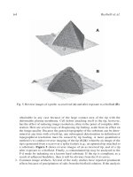
Fig. 8 Illustration of the various recording modes of the PFM: (a) to image a surface in the contact mode, the
focus holding the probe particle is scanned over the surface laterally. This can be done either by maintaining a
constant distance to the support (solid line) or by using a feedback, moving the focus up and down (dashed line)
to maintain a constant force between probe and sample. (b) In the PFM tapping mode the focus is approached
to the sample in each image point, and upon contact is retracted a predefined distance. (c) Three-dimensional
SPT of a sphere bound to a diffusing membrane particle: the laser trap is held steady, and the Brownian motion
of the diffusing particle is used to record the interaction with the environment.
the optical axis, i.e., vertically (+z) away from the surface. The displacement results
in a further decrease of the two-photon fluorescence intensity. An image of the surface
topography is acquired by recording the fluorescence intensity while raster scanning an

area. If the bead is displaced too far away from the focus, it escapes the trapping potential.
Therefore, the height of the object has to be smaller than the trapping range of the laser
trap, which is about 0.8 μm.
The vertical working range is substantially extended by using a feedback circuit that
drives the piezo-mounted objective lens up or down maintaining a constant fluorescence
intensity and constant position of the probe in the laser trap, thus creating a constant
force mode. Because of the large mass of the objective lens, the response time of the
feedback is limited.
While these scan modes rely on the two-photon fluorescence intensity as a measure for
the axial displacement of the probe in the trap, it is advisable to simultaneously record the
signals from the quadrant detector as well. These signals provide information about the
three-dimensional displacement of the probe and, taken together, help to reveal possible
scan artifacts in the normal topographic image.
2. Tapping Mode
In the tapping mode, the sphere trapped by the laser beam is brought repeatedly into
contact with the surface (Fig. 8b). The PFM tapping mode can be compared to the force–
scan volumes acquired by conventional SFM(Radmacher et al., 1996). In each pointof an
image, the surface is approached while recording the two-photon fluorescence intensity.
When the fluorescence intensity decreases below a preset set fraction of the intensity
210 Pralle and Florin
measured for the free sphere, the sphere is retracted a fixed distance and moved to the next
point. The tapping mode enables the measurement of virtually vertical slopes. Because
the contact times and forces are reduced, the spheres are less often lost due to nonspecific
adhesion to the cell surface. The vertical range in the tapping mode is limited either by
the working range of the driving piezo, i.e., 100 μm, or by spherical aberration effects,
which restrict the range of stable trapping for larger distances from the coverslip surface.
The tapping mode feedback is implemented via a DSP board and by a computer that
also displays the image and individual force scans. A reference fluorescence intensity
for the free sphere is measured in each point to avoid image distortion due to bleach-
ing of the sphere and laser intensity variations in the sample plane. The height of the

endpoint of each force scan depends on the imaged topography. The probe is retracted
at constant distances from the last contact with the surface, enabling the PFM to climb
up the extremely steep edge, without the need for extremely long and time-consuming
force scans. The elasticity of the surface is computed from the slope of the two-photon
fluorescence intensity decrease. Again, using the QPD to detect the forward-scattered
light, the lateral displacement of the sphere upon contact can be recorded simultaneously.
3. Fast Three-Dimensional Single-Particle Tracking
To measure the local environment of single-membrane proteins, no active scanning is
necessary, but the thermal position fluctuations of a sphere in a weak trapping potential.
The rms thermal position noise in a trapping potential of 2 μN/m is ≈45 nm. Measuring
this motion precisely using the forward scattered light allows recording of the three-
dimensional diffusion on the cell surface with high temporal resolution. The free trapping
potential is plotted to visualize the volume accessible to the bead. Any deviations thereof
are due to interacting potentials or obstructions such as a surface of stable object or
immobile membrane components. The local viscousdrag can be determinedby analyzing
the motion along the track.
G. Sample Preparation
It is essential to prepare the sample surfaces as cleanly as possible to minimize the
nonspecific interaction between the probe and the sample and to avoid collecting small
biological particles like vesicles in the laser trap. The cellular samples are prepared as
follows: Baby-hamster kidney (BHK-21) cells are grown, according to standard cell
culture procedures, in a tissue culture flask with supplemented Glasgow(G)-MEM and
passaged every 2–3 days. The hippocampal neurons are extracted from 18-day-old rat
embryos, plated on poly-
L-lysine-coated coverslips in a dish that was preincubated with
glia cells and grown at 37
◦
C and 5% CO
2
in N

2
culture medium (Goslin and Banker,
1991). Circular glass coverslips (11 mm) are used as substrate for the cells. These are
cleaned and sterilized (either autoclaved or washed in acetone/ethanol and dried in sterile
air). The cells, BHK fibroblasts or hippocampal neurons, are plated at low density on
the coverslips and allowed to grow 3–5 days. At this stage, the early development of the
major processes and the growth cone morphology of the neurons can be studied.
9. Cellular Membranes Studied by PFM 211
For imaging of living cells, the cells are washed and imaged in filtered culture medium
the same. In the case of the neuronal cells, it is advisable to use the culture medium from
the dish in which the cells had been growing to maintain the exact composition of the
medium during the experiment. For the experiments on fixed cells, the cells are washed
twice in PBS, fixed in 1% glutaraldehyde for 10 min at room temperature, washed three
times in PBS, and incubated for 10 min in 50 mM NH
4
Cl to block any free aldehyde
groups. Cells for live imaging are washed again in PBS containing 10 mg/ml FSG. The
scanning experiments are carried out in culture medium for living cells and in PBS for
fixed cells. In both cases, 10 mg/ml FSG is added to the solution and the microscope
stage is heated to 35
◦
C. All solutions should be filtered through 0.1-μm SuporeAcrodisc
filters (Gelman Sciences, www.pall.com/gelman).
To study nonendogenous membrane proteins, the cells can be either transfected 12–
14 h prior to theexperiment using a trasporter such as lipofectamine(Gibco,www.lifetech.
com) or infected using a retrovirus-based system, like the adenovirus. In any case it is
useful to cotransfect the cells with a cytoplasmic green fluorescent protein (E-GFP) to
facilitate the search for successfully transfected cells. The virus system provides the ad-
vantages of being very reproducible, yielding high ratios of infected cells and disturbing
the composition of the plasma membrane the least.

References
Allersma, M. W., Gittes, F., deCastro, M. J., Stewart, R. J., and Schmidt, C. F. (1998). Two-dimensional
tracking of ncd motility by back focal plane interferometry. Biophys. J. 74(2), 1074–1085.
Ashkin, A., Dziedzic, J. M., Bjorkholm, J. E., and Chu, S. (1986). Observations of a single-beam gradient
force optical trap for dielectric particles. Opt. Lett. 11, 288–290.
Ashkin, A., Sch¨utze, K., Dziedzic, J. M., Euteneuer, U., and Schliwa, M. (1990). Force generation of organelle
transport measured in vivo by an infrared laser trap. Nature 428, 346–348.
Cherry, R. J. (1992). Keeping track of cell surface receptors. Trends Cell Biol. 2, 242–244.
Dabros, T., Warszynski, P., and van den Ven, T. G. M. (1994). Motion of latex spheres tethered to a surface.
J. Colloids Surf. B 4, 327–334.
Dai, J., and Sheetz, M. P. (1995). Mechanical properties of neuronal growth cone membranes studied by tether
formation with laser optical tweezers. Biophys. J. 68(3), 988–996.
De Brabander, M., Nuydens, R., Ishihara, A., Holifield, B., Jacobson, K., and Geerts, H. (1991). Lateral
diffusion and retrograde movements of individual cell surface components on single motile cells observed
with nanovid microscopy. J. Cell Biol. 112, 111–124.
Edidin, M., Kuo, S. C., and Sheetz, M. P. (1991). Lateral movements of membrane glycoproteins restricted by
dynamic cytoplasmic barriers. Science 254, 1379–1382.
Evans, E. A. (1983). Bending elastic modulus of red blood cell membrane derived from buckling instability
in micropipette aspiration tests. Biophys. J. 43(1), 27–30.
Evans, E. A., and La Celle, P. L. (1975). Intrinsic material properties of the erythrocyte membrane indicated
by mechanical analysis of deformation. Blood 45(1), 29–43.
Finer, J. T., Simmons, R. M., and Spudich, J. A. (1994). Single myosin molecule mechanics: piconewton forces
and nanometre steps. Nature 368, 113–118.
Florin, E L., Pralle, A., H¨orber, J. K. H., and Stelzer, E. H. K. (1997). Photonic Force Microscope based on
optical tweezers and two-photon excitation for biological Applications. J. Struct. Biol. 119, 202–211.
Florin, E. L., Pralle, A., Stelzer, E. H. K., and Hoerber, J. K. H. (1998). Photonic force microscope calibration
by thermal noise analysis. Appl. Phys. A 66, S75–S78.
Ghislain, L. P., and Webb, W. W. (1993). Scanning-force microscope based on an optical trap. Opt. Lett. 18,
1678–1680.
212 Pralle and Florin

Gittes, F., and Schmidt, C. F. (1998). Interference model for back focal plane displacement detection in optical
tweezers. Opt. Lett. 23, 7–9.
Goslin, K., and Banker, G. (1991). “Culturing Nerve Cells.” M.I.T. Press Cambridge, MA.
Grimellec, C. L., Lesniewska, E., Cachia, C., Schreiber, J. P., Fornel, F. d., and Goudonnet, J. P. (1994).
Imaging of the membrane surface of MDCK cells by atomic force microscopy. Biophys. J. 67, 36–41.
H¨aberle, W., H¨orber, J. K. H., and Binnig, G. (1991). Force microscopy on living cells. J. Vac. Sci. Technol.
B9 2, 1210–1213.
Hertz, H. M., Malmqvist, L., Rosengren, L., and Ljungberg, K. (1995). Optically trapped non-linear particles
as for scanning near-field optical microscopy. Ultramicroscopy 57, 309–312.
Jacobson, K., Sheets, E. D., and Simons, R. (1995). Revisiting the fluid mosaic model of membranes. Science
268, 1441–1442.
Kusumi, A., Sako, Y., and Yamamoto, M. (1993). Confined lateral diffusion of membrane receptors as studied
by single particle tracking (nanovid microscopy). Effects of calcium-induced differentiation in cultured
epithelial cells. Biophys. J. 65(5), 2021–2040.
Malmquist, L., and Hertz, H. M. (1992). Trapped particle optical microscopy. Opt. Commun. 94, 19–24.
Mehta, A. D., Finer, J. T., and Spudich, J. A. (1998). Reflections of a lucid dreamer: Optical trap design
considerations. In “Methods in Cell Biology” (M. Sheetz, ed.), Vol. 55, pp. 47–69. Academic Press, San
Diego.
Pralle, A., Florin, E. L., Stelzer, E. H. K., and Hoerber, J. K. H. (1998). Local viscosity probed by photonic
force microscopy. Appl. Phys. A 66, S71–73.
Pralle, A., Keller, P., Florin, E L., Simons, K., and H¨orber, J. K. H. (2000). Sphingolipid—Cholesterol rafts
diffuse as small entities in the plasma membrane of mammalian cell. J Cell Biol. 148, 997–1007.
Pralle, A., Prummer, M., Florin, E L., Stelzer, E. H. K., and H¨orber, J. K. H. (1999). Three-dimensional
position tracking for optical tweezers by forward scattered light. Micro. Res. Technol. 44, 378–386.
Radmacher, M., Fritz, M., Kacher, C. M., Cleveland, J. P., and Hansma, P. K. (1996). Measuring the viscoelastic
properties of human platelets with the atomic force microscope. Biophys. J. 70, 556–567.
Radmacher, M., Tillmann, R. W., Fritz, M., and Gaub, H. E. (1992). From molecules to cells: Imaging soft
samples with the atomic force microscope. Science 257, 1900–1905.
Sako, Y., and Kusumi, A. (1995). Barriers for lateral diffusion of transferrin receptor in the plasma membrane
as characterized by receptor dragging by laser tweezers: fence versus tether. J. Cell Biol. 129(6), 1559–1574.

Sasaki, K., Shi, Z. Y., Kopelman, R., and Masuhara, H. (1996). Three-dimensional pH microprobing with an
optically-manipulated fluorescent particle. Chem. Lett. 2, 141–142.
Singer, S. J., and Nicolson, G. L. (1972). The fluid mosaic model of the structure of cellmembranes. Science
175(23), 720–731.
Stout, A. L., and Webb, W. W. (1998). Optical force microscopy. In “Methods in Cell Biology” (M. Sheetz,
ed.), Vol. 55, pp. 47–69. Academic Press, San Diego.
Svoboda, K., and Block, S. M. (1994). Biological applications of optical forces. Annu. Rev. Biophys. Biomol.
Struct. 23, 247–285.
Tomishige, M., and Kusumi, A. (1999). Compartmentalization of the erythrocyte membrane by the membrane
skeleton: inter compartmental hop diffusion of bond 3. Mol. Biol. Cell 10(8), 2475–2479.
Vaz, W. L. C., and Almeida, P. F. F. (1993). Phase topology and percolation in multiphase bilayers: Is the
biological membrane a domain mosaic. Curr. Opin. Struct. Biol. 3,
482–488.
Visscher, K., and Brakenhoff, G. J. (1992). Theoretical study of optically induced forces on spherical particles
in a single beam trap. I. Rayleigh scatterers (cellular micromanipulator). Optik 89, 174–180.
Zhang, F., Lee, G. M., and Jacobson, K. (1993). Protein lateral mobility as a reflection of membrane
microstructure. Bioessays 15(9), 579–588.
Zocchi, G. (1996). Mechanical measurement of the unfolding of a protein. Europhys. Lett. 35, 633–638.
CHAPTER 10
Methods for Biological Probe Microscopy
in Aqueous Fluids
Johannes H. Kindt, John C. Sitko, Lia I. Pietrasanta,
∗
Emin Oroudjev, Nathan Becker, Mario B. Viani,
†
and Helen G. Hansma
Department of Physics
University of California
Santa Barbara, California 93106
I. Introduction

II. Substrates/Surfaces
III. Basic Methods for Atomic Force Microscopy in Aqueous Fluids
A. Imaging without an O Ring
B. Imaging with an O Ring
C. Removing Bubbles from the Cantilever
D. Imaging Modes
E. Imaging Parameters
F. Cantilevers
G. Effects of Different Aqueous Solutions on AFM Imaging
H. When To Image in Fluid
I. When Not To Image in Fluid
IV. Molecular Force Probing
V. Advanced Fluid Handling
A. Principle of Operation
B. DNase Digesting DNA—A Fluid-Handling Example
C. Outlook
VI. Conclusion
References
∗
Current address: Laboratorio de Electr´onica Cu´antica, Departamento de F´ısica, Pabell´on I - Ciudad
Universitaria, C1428EHA Buenos Aires, Argentina.
†
Current address: Asylum Research, Santa Barbara, CA 93117.
METHODS IN CELL BIOLOGY, VOL. 68
Copyright 2002, Elsevier Science (USA). All rights reserved.
0091-679X/02 $35.00
213
214 Kindt et al.
I. Introduction
It is easier and often faster to image biological samples in air than in aqueous fluid. But

imaging in aqueous fluids is almost always preferable if one wants to see biomaterials in
near-physiological environments. When imaging in fluid, one sees biomaterials not only
under conditions where their structures are native but also under conditions where the
biomaterials retain their biological activity. This activity can be monitored and, using ad-
vanced fluid handlingtechniques, investigated under changing environmental conditions.
It has been said that atomic force microscopy (AFM) is unnatural because the atomic
force microscope (AFM) looks at biomaterials on surfaces instead of in test tubes. The
development of biological AFM has also been handicapped by “test tube biology,”
because in vitro biological systems have been developed to work in test tubes, while the
AFM looks at biological systems on surfaces. But living systems are filled with surfaces,
especially membranes. Therefore surfaces are arguably more relevant biologically than
test tubes. In fact, AFM may be a leader in a new field, Surface Biology, which will grow
into a major research area in the new century.
This article covers methodology for using AFMs and other probe microscopes with
which the authors are familiar. These areDigital Instruments scanning probe microscopes
(SPMs) and the Asylum Research Molecular Force Probe (MFP). The MFP is a new
instrument optimized for molecular pulling experiments of the type shown in Fig. 1.
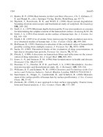
Fig. 1 A single molecule of overstretched DNA. This graph shows a force measurement of a single tethered
molecule of Lambda Digest DNA showing the B–S and the melting transition. Arrowheads indicate pulling
direction as follows: DNA stretch is
 and DNA relaxation is . During the extension of the molecule (red
trace), the DNA first goes through the B–S transition (the plateau) and then melts to single-stranded DNA
(ss-DNA) at a higher force. During relaxation of the molecule (blue trace), the DNA does not reanneal, so
the curve is a simple freely jointed chain, indicative of ss-DNA. The traces were made at a pulling speed of
1 mm/s. Data courtesy of H. Clausen-Schaumann and R. Krautbauer, Gaub Lab, LMU-M¨unchen. Data were
obtained with a cantilever from Park Scientific Microlevers on a Molecular Force Probe from Asylum Research
(). (See Color Plate.)
10. Biological Probe Microscopy in Aqueous Fluids 215
II. Substrates/Surfaces
“Substrates” in this context are the surfaces that biomaterials are placed on for AFM

imaging. Common substrates for biological AFM are mica and glass. Glass is flat enough
for imaging cells but is generally too rough for easy visualization of DNA, especially
under fluid.
Biomaterials such as DNA and proteins are usually imaged on mica, which has a root-
mean-square roughness of only 0.06 ± 0.01 nm (Hansma and Laney, 1996). Silylated
mica and other treated micas such as Ni(II)-mica (Bezanilla et al., 1994; Hansma and
Laney, 1996)and Mg(II)-mica are also used. AP-mica isthe most common ofthe silylated
mica substrates (Bezanilla et al., 1995; Lyubchenko et al., 1992); its RMS roughness of
0.09 ± 0.01 nm is only slightly rougher than mica.
The biomaterials of interest need to adhere at least weakly to the substrate if they are
to be imaged well in aqueous fluid.
III. Basic Methods for Atomic Force Microscopy
in Aqueous Fluids
A. Imaging without an O Ring
This is the default method for many SPMs, and it is an optional method when using
the MultiMode SPM.
Given the importance of biological imaging in fluid, one wants to be able to image in
fluid as simply as possible. One thing that makes biological imaging easier, when using
the Digital Instruments MultiMode AFM, is to leave out the O ring. One can usually
image for about an hour under a drop of fluid before evaporation becomes a problem.
There are at least two ways to set up samples for imaging in fluid. Often one can simply
place a drop of 30–35 μL, containing the biomaterial of interest, on the cantilever in the
fluid cell and then quickly turn over the fluid cell and insert it into the AFM over the
substrate. Of course one wants to be sure beforehand that the cantilever will not crash onto
the substrate, so one may want to do a “coarse approach” with the dry cantilever + fluid
cell + substrate in the AFM before adding the sample solution.
If one wants to image for longer than an hour, one will want to add a few microliters
(μL) of water or buffer to the fluid cell periodically. One can do this with a syringe or
a microliter pipetter, inserted into the space between the fluid cell and the sample. Or,
when using a MultiMode AFM, one can inject fluid into one of the syringe ports in the

fluid cell.
Sometimes one wants the solution above the sample to be purely buffer solution,
without the biomolecules or other biomaterials that are in the solution. In these cases,
one can place the sample on the substrate in the AFM in a volume of 1–5 μL, place a
buffer drop of 30–35 μL on the cantilever in the fluid cell, and then quickly turn over the
fluid cell onto the substrate as in the example above. When using a very small sample
volume, one will of course want to be speedy about getting the sample submerged in
buffer on the cantilever before the sample on the substrate dries up. The sample can also
216 Kindt et al.
be rinsed to remove loosely bound biomaterials before placing the cantilever with buffer
solution over it.
If one wants to change fluids while the sample is in a MultiMode AFM, it is usually
best to work with an O ring. Here, too, however, one can do limited fluid changing
without using an O ring. One way to do this is to have two 1-mL syringes in the ports of
the MultiMode fluid cell—one empty syringe and one filled with the new solution. The
old solution can be sucked into the empty syringe, followed by a cautious injection of
new solution from the filled syringe— ∼50 μL will be sufficient. Repeating this a few
times will give a fairly complete exchange of fluid—but one must be careful not to inject
too much fluid, or it will flow over the edge of the sample and onto the scanner.
Similarly, one can change fluid in other open fluid cells by using syringes with needles
for injecting and removing solutions in the space between the cantilever and the substrate.
A much finer system for pumping fluids into the fluid cell during imaging has been
developed by our group, using computer-controlled fluid changes and microliter volume
injections that can be carried out with little or no disruption of the image whose capture
is in progress. We will discuss this option later.
B. Imaging with an O Ring
For more serious imaging with the MultiMode AFM under a series of fluids, the O
ring is unavoidable. One can improve the O ring somewhat by slicing off the outer edge
with a razor blade or scalpel to decrease the outer diameter of the O ring. Much better
O rings with a new cross section have been designed by Johannes H. Kindt at UCSB.

Hopefully these will soon become commercially available to the AFM community.
With an O ring to enclose the fluid cell, one will want to think about automating the
flow of fluids into and out of the fluid cell. This can be done either with the computer-
controlled system described later or with a gravity flow system using syringe barrels and
valves as described by Thomson et al. (1996). The flow rate for this system is measured
by collecting the effluent into a beaker on an electronic balance.
C. Removing Bubbles from the Cantilever
Air bubbles are a problem when they sit on the cantilever. If one is having imaging
problems, it is wise to check for bubbles, which can cause imaging problems in fluid.
Sometimes air bubbles can be removed simply by lifting the fluid cell and lowering it
down again over the sample. Or the fluid cell can be removed from the AFM and tapped
gently to dislodge bubbles. Another way to dislodge bubbles is to flush fluid in and out
of the fluid cell with a syringe attached to the port of the fluid cell.
One can also easily degas solutions before use, if there is a persistent problem with air
bubbles. To degas a solution, pull it into a syringe, hold a piece of parafilm over the end
of the syringe with your finger, and pull on the plunger of the syringe until air bubbles
form. Tap the syringe against the edge of the lab bench while pulling on the plunger to
dislodge bubbles from the walls of the syringe, and they will rise into the air space above
the solution. Bubbles will, of course, be a problem whenever one injects cold fluids into
the fluid cell, so temperature equilibration of fluids is important.
10. Biological Probe Microscopy in Aqueous Fluids 217
D. Imaging Modes
The two standard AFMimaging modes are tappingand contact. Our labs almostalways
uses the tapping mode, which reduces lateral forces. For some samples, the contact mode
is preferred. It is often easier to see substructural detail in the contact mode when imaging
flat samples where lateral forces are small. For example, two-dimensional protein arrays,
including membrane protein arrays, are usually imaged in the contact mode (Czajkowsky
and Shao, 1998; Engel et al., 1997; M¨uller et al., 1998; Yang et al., 1994), although the
tapping mode AFM can give comparable resolution in the hands of an experienced user
(Moller et al., 1999).

E. Imaging Parameters
In the late 1980s, a newcomer to the AFM field said he had expected to find that using
the AFM was rather like using a toaster (Hermann Gaub, personal communication).
Instead, he found it to be more like playing a violin. Although the AFM is becoming more
toaster-like with its new improvements and more user experience, it is still somewhat
violin-like. Therefore the user will find it useful to experiment with gains, setpoint, scan
speed, drive frequency, and drive amplitude to find the best conditions for each new
sample. The details presented in the following paragraphs about imaging parameters are
to be used as a guide, not as a strict protocol.
When determining the frequency response for cantilevers in fluid, automatic tuning
methods may not work. A plot of amplitude versus frequency shows multiple peaks in
fluid. The highest peak does not necessarily produce optimal imaging. With experience,
one usually finds that a particular location in these peaks gives good images. Thislocation
is often 5–10% below the peak frequency of the selected peak. A good technique for
newcomers is to check the imaging quality at or slightly below the peak frequency of
a few of the peaks until satisfactory results are obtained. If imaging quality starts to
degrade while using the same cantilever, one can check the cantilever tuning again and
readjust the drive frequency. Our lab typically uses 100-micron-long, narrow, V-shaped,
silicon–nitride cantilevers in Plexiglas fluid cells. With these home-made Plexiglas fluid
cells, the optimal peak frequency is typically close to 13 kHz. With glass fluid cells, the
primary cantilever oscillations are at lower frequencies, near 9 kHz. These oscillations
are all in the envelope of the thermal resonance frequency for the cantilever in fluid
(Schaffer et al., 1996).
After the correct frequency is determined, the gains can be optimized. One can start
scanning with the integral gain set at 1.2 and the proportional gain twice as large. With
these values one can usually tell whether an image is obtainable or if one needs to change
the frequency or the tip. Proportional gains are significantly less sensitive than integral
gains, so first the integral gain must be adjusted only until the image is optimal. Then
the proportional gain must be adjusted. This gain ends up being about two or three times
the integral gain. We commonly use an integral gain between 1 and 3 in fluid, though

we have used much higher gains on occasion.
The optimum imaging setpoint is selected by lifting off the surface completely while
scanning, then slowly approaching until an image is formed. With dry AFM, pushing
harder on the sample will often give a sharper image. In aqueous AFM, samples can be
218 Kindt et al.
particularly soft, so minimal forces are often optimal. One may want to rescan the same
area with a larger scan size to ensure one has not scraped the surface.
The imaging setpoint correlates with the drive voltage. In general smaller drive
voltages are good for imaging relatively flat samples such as DNA and proteins on
mica, while larger drive voltages are good for imaging relatively thick, sticky, or soft
samples such as cells. With small-drive voltages, the setpoints for low-force imaging
will be 0.5 V or less; with large-drive voltages, the setpoints for low-force imaging will
be 1–2 V or higher.
In general, the scanning speed does not need to be changed when going from dry to
aqueous samples. We usually use a scan speed of 2–4 Hz.
F. Cantilevers
As mentioned earlier, our lab typically used 100-micron-long, narrow, V-shaped,
silicon–nitride cantilevers. EBD tips, oxide-sharpened Si–N tips and normal pyrami-
dal Si–N tips have all been used successfully. Before fluid tapping was possible, we
observed that EBD tips gave less sample damage (Hansma et al., 1993).
The 200-micron-long, wide V-shaped cantilevers have a similar spring constant to the
100-micron narrow cantilevers. Their larger size makes them easier for beginners to use,
and we have used them successfully for many samples. These 200-micron cantilevers are
probably preferable to the 100-micron cantilevers for users who do not have a scanner
with “vertical engage” suchas the original MultiModescanners from Digital Instruments.
For older MultiMode scanners that need to be leveled manually, it is easier to get the
longer cantilevers level enough with respect to the surface; with the shorter cantilevers,
even a small sample tilt can cause the corner of the cantilever chip to hit the sample
instead of the cantilever tip. Feeler gauges are useful for leveling these older scanners.
Other soft cantilevers for imaging in fluid are 400-micron-long rod-shaped silicon can-

tilevers and V-shaped silicon cantilevers from Park Scientific (now ThermoMicroscopes,
Sunnyvale, CA).
G. Effects of Different Aqueous Solutions on AFM Imaging
Much of the challenge with biological AFM in fluid is in finding a good aqueous buffer
solution that supports the biological activity of interest and also keeps the biomolecules
well enough immobilized on the substrate for good imaging but not so tightly bound
as to be inactive. In our group we explored and succeeded in imaging in liquid differ-
ent biological macromolecules such as laminin, chaperonins, DNA, and DNA–protein
complexes.
We investigated the three-dimensional arrangement and dynamic motion of
laminin-1 (Ln-1) molecules (Chen et al., 1998). Laminins are a family of extracellu-
lar matrix glycoproteins that play an active role in tissue development and maintenance.
Four different buffers at pH 7.4 were used: high-salt MOPS buffer (20 mM MOPS,
5mM MgCl
2
, 150 mM NaCl), low-salt MOPS buffer (20 mM MOPS, 25 mM NaCl,
5mM MgCl
2
), PBS in 5 mM MgCl
2
(10 mM phosphate buffer, 2.7 mM KCl, 137 mM
10. Biological Probe Microscopy in Aqueous Fluids 219
NaCl), and Tris buffer (50 mM Tris, 150 mM NaCl, 5 mM MgCl
2
). The two MOPS
buffers (low-salt and high-salt) were the best for imaging substructures in individual
Ln-1 molecules. The lower panels in Fig. 3 show the flexibility and mobility of Ln-1
arms in high-salt MOPS buffer (physiologicalconditions). Sometimes, imaging in a high-
salt buffer was not as easy as imaging in a low-salt buffer. The images appeared less well
defined, perhaps because the molecules were more weakly attached to the mica. Imaging

Ln-1 in PBS or Tris buffer was very difficult, and the images were poor. In contrast to the
successful imaging of Ln-1 in fluid, other basement-membrane macromolecules such
as collagen IV and heparan sulfate proteoglycan could not be imaged in the previously
cited buffers, though they gave good images in air (Chen and Hansma, 2000).
Another example of proteins imaged in solution without additional treatment such as
fixation is the Escherichia coli chaperonin GroEL and its co-chaperonin GroES. These
proteins play important roles in helping proteins reach their native states. We were able
to scan the same sample region without excessively disturbing the array of either the
GroEL or the GroES molecules. The central channel of the protein was resolved in many
of the molecules. The best results were obtained when the protein arrays were imaged in
50 mM Hepes (pH 7.5), 50 mM KCl, and 10 mM MgCl
2
. These preliminary results with
a commercial AFM were followed by analyses of protein dynamics with a prototype
small-cantilever AFM (Viani et al., 2000).
To study biological processes such as DNA–protein interactions in fluid with the
AFM, one has to compromise between strongly bound DNA, essential for good imaging
conditions, and loosely bound DNA, required for reactions with other molecules such
as enzymes. We have found, after exploring several buffers containing salts of divalent
inorganic cations, that DNA molecules bindtightlyenough to mica if the solution contains
1mM concentrations of Ni(II), Co(II), Zn(II), or Mn(II) (Hansma and Laney, 1996). This
finding was valuable for demonstrating the activity of E. coli RNA polymerase (RNAP)
on mica (Kasas et al., 1997). With varying Zn
2+
concentration in the buffer solution, the
DNA molecules bound loosely enough to be translocated by the RNAP and also with
sufficient strength to be imaged with the AFM (e.g., Fig. 2). Although our labs have
favored the use of divalent transition metal salts, the Bustamante lab has successfully
imaged RNAP complexes in buffers without these salts (Bustamante et al., 1999; Guthold
et al., 1999). This is another example of the “violin-playing” nature of AFM imaging at

present.
We have observed other DNA–enzyme processes in the AFM, including reactions
of DNA with other polymerases (Argaman et al., 1997; Hansma et al., 1999) and with
DNaseI (Bezanilla et al., 1994; Hansma, 2000; Hansma et al., 2000). DNA degradation
by DNaseI is a robust process in the AFM that makes it useful for testing new instru-
mentation such as the automated fluid-handling system of Fig. 4. After stable imaging
in the presence of Ni(II), the buffer containing Mn(II) (the divalent cation required for
the enzyme activity) and the DNaseI solution were injected with this system, yielding
the results shown in Fig. 5.
Observing other DNA–enzyme interactions is an avenue of progress that provides
many opportunities for new development in the instrumentation and new strategies in
the imaging conditions.
220 Kindt et al.
Fig. 2 Two active complexes of DNA with RNAP under fluid in an AFM. E. coli RNAP transcription
complexes were prepared with a 1047-bp DNA template (Guthold et al., 1999; Kasas et al., 1997). (A), (B),
and (C) each show a series of four consecutive images at 42-s intervals. (A) DNA strands move near the surface
in Zn(II) buffer. (B) 3.5–6 min after the last image in (A). RNAP transcribes and/or detaches from DNA strands
after NTPs are introduced. (C) 6–8 min after the last image in (B); Zn(II) buffer is reintroduced. Note that the
image quality deteriorates in Zn(II)-free buffer and improves as Zn(II) buffer is reintroduced [see Hansma and
Laney (1996)]. DNA images are 310 nm ×330 nm. (See Color Plate.)
Fig. 3 AFM imaging of laminin molecules in air shows submolecular structure in the laminin arms (top
row). In the sequential images, a single laminin molecule in aqueous solution waves its arms (bottom row).
(See Color Plate.)
10. Biological Probe Microscopy in Aqueous Fluids 221
Fig. 4 The setup of the fluid-handling system. On the left are the pump-modules that inject fluid from
different source solutions. On the right are the additional pump-modules sucking solution from an open fluid
cell at the same rate. In the center is the fluid chamber around the sample with the cantilever above the sample.
(See Color Plate.)
H. When To Image in Fluid
Fluid imaging is essential if one wants to see something happening, such as moving

DNA molecules in the complexes with RNA polymerase in Fig. 2 (Hansma, 1999;
Kasas et al., 1997) or the motion of the laminin arms in Fig. 3. Another useful type of
AFM in fluid is force mapping or force–volume (FV) imaging (Brown and Hoh, 1997;
Radmacher et al., 1994) (Fig. 6). This FV image of three synaptic vesicles with dark
spots in their centers shows darker and lighter regions that correspond to harder and
softer regions, respectively (Laney et al., 1997). We were surprised to find that these
vesicles were harder in their centers than at their edges, unlike most cells and other soft
things (imagine, for example, a pillow). One can see that the vesicle centers are harder
or stiffer than their peripheries because they are dark like the mica surface (though not
nearly as hard as mica).
I. When Not To Image in Fluid
One does not want to get carried away with imaging in fluid, though, to the exclusion
of imaging in air. It is of course usually easier to get stable images in air than in fluid,
and air images also often have better resolution. For example, in Fig. 3, the images of
laminin in fluid show the arms moving, but the images in air show the substructure in
the laminin arms in much greater detail (Chen et al., 1998).
Another example where imaging in air has proved to be more useful than imag-
ing in fluid is the Ni(II)-mediated condensation of the DNA, poly (dG–dC)
∗
(dC–dG)
222 Kindt et al.
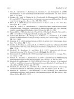
Fig. 5 Enzymatic degradation of single DNA molecules in the AFM. A field of DNA molecules (0.5 μg/
mL of BlueScript plasmid DNA) in a buffer containing 20 mM Hepes, 5 mM MnCl
2
, pH 7.6, continuously
pumped at 5 μL/s. After the injection of DNaseI into the same buffer, the degradation of the molecules can
be observed; arrows indicate frame and position in frame where the 10-μL injections occurred. The circles
highlight new cuts in DNA molecules. The scan size is 1 μm × 1 μm; the z range is 7 nm. All imaging was
done on a Nanoscope III Multimode-AFM (Digital Instruments). The microscope was operated in the fluid
tapping mode using cantilever oscillation frequencies between 10 and 20 kHz. (See Color Plate.)

Fig. 6 Three cholinergic synaptic vesicles. Height image (left) and force–volume (FV) image (right) of
three synaptic vesicles from the electric organ of Torpedo. The centers of the vesicles are harder or stiffer than
the edges of the vesicles (see Laney et al., 1997). (See Color Plate.)
10. Biological Probe Microscopy in Aqueous Fluids 223
Fig. 7 These condensed DNA structures in air (left) and fluid (right) are similar. The side loops on these
DNA condensates can be imaged more stably in air. Poly (dG–dC)
∗
(dG–dC) condensed with 1 mM NiCl
2
to
form loopy toroids. Left: A typical field of condensates was imaged with tapping mode AFM in air. Right:
These three toroids were found in aqueous tapping mode AFM images. The scale bar applies to all images.
(GC-DNA)(Fig. 7, (Hansma 1999; Sitko, in preparation)). With this system, the observed
structures were similar in air and in fluid. Because the DNA condensates bound strongly
and irreversibly to the mica, they did not move or condense further during AFM in fluid.
Therefore it was easier and no less useful to image these condensates in air instead of in
fluid.
IV. Molecular Force Probing
A relatively new application for probe microscopy in fluid deserves special mention.
One of the most dramatic examples of this new application is the unfolding of individual
titin protein molecules (Fisher et al., 1999; Rief, Gautel et al., 1997). Other examples
include tensile pulling of double-stranded DNA molecules (Lee et al., 1994) and single
polysaccharide molecules (Rief, Oesterhelt et al., 1997), measuring the strength of single
covalent bonds (Grandbois et al., 1999)and ligand–receptor orligand–ligand interactions
(Dammer et al., 1995, 1996; Florin et al., 1994). This AFM application is sometimes
called force spectroscopy (Rief, Oesterhelt et al., 1997). Hereit is referred to asmolecular
force probing (MFPing) to distinguish it from probe microscopic techniques that require
scanning.
MFPing essentially involves measurements of force versus distance characteristics
for single or multiple molecules stretched between the cantilever tip and the substrate in

the AFM contact mode. The molecules being probed are attached through covalent or
224 Kindt et al.
noncovalent interactions to the substrate and to the tip of the cantilever. A large array of
techniques can be employed to achieve this goal. Usually, the tip of the AFM probe is first
pressed against substrate, which has thematerial of interestdeposited onto it. After a short
incubation time (on theorderof 1 s, to allowthe molecules of interest bindtothe tip) single
or multiple pulls are performed. Both the tip and the substrate can be modified and/or
functionalized to allow more specific attachment of material of interest to both working
surfaces (Lee et al., 1994; MacKerell and Lee, 1999; Rief, Oesterhelt et al., 1997).
During each pull, the tip and cantilever move away from and toward the substrate.
The primary form of the raw data from an MFP experiment is the deflection of the
laser beam versus the distance of cantilever movement in the z direction. These data
can be transformed into force versus distance plots using the Hooke’s law formula
f (Force) = kx where x is the distance that the tip of cantilever was deflected and k
is the spring constant for the cantilever. The spring constant for the cantilever can be
estimated by a few different methods (Cleveland et al., 1993; Sader et al., 1995) if the
instrument used for pulling does not have a built-in system for estimating the spring
constant. One also calibrates the microscope to find the sensitivity of the cantilever,
which is piezo-voltage per nanometer of cantilever deflection on a hard surface. This
can be done by first manually approaching the surface with the tip and then pressing the
tip against the surface until it is sharply deflected. Then one can perform a single pull in
the away-then-back-to-the-surface direction and record the deflection of the laser beam
versus the distance of the cantilever movement. This graph serves as a calibration curve
for cantilever deflection values. When these calibrations are done, the MFP is ready for
actual pulling experiments. After data are converted into force versus distance graphs
as in Fig. 1, the best fitting model can be found for each separate pulling event (for
example, worm-like chain model for titin domains unfolding or DNA stretching). From
this model one can calculate corresponding contour lengths and persistence lengths for
each observed event (Fisher et al., 1999).
Numerous modifications of MFPing can be used to study intermolecular as well as

intramolecular interactions. Elasticity of biopolymers, protein, and nucleic acid folding,
interactions between biomolecules and receptor–ligand interactions, and forces of cova-
lent and noncovalent bonds are a few examples of problems that can be studied with the
MFP technique. Although almost any standard AFM can be used to perform some MFP
experiments, the molecular force probe (MFP) from Asylum Research (Santa Barbara,
CA) is dedicated specifically for nano-pulling experiments. The MFP has both hardware
and software advantages over conventional AFM. The main hardware advantage is the
improved control over the z position of the cantilever relative to the sample due to an
absolute position sensor. This can be crucial in pulling experiments as repetitive pulling
events often have to be performed without touching the substrate while, at the same
time, approaching very close to the substrate. This is also a major software advantage
of the MFP as compared to the AFMs we are acquainted with: that the software can
perform repetitive molecular pulls without touching the substrate between pulls. The
MFP’s IGOR software (Wavemetrics, Lake Oswego, OR) can also be easily modified
for specific experiments through macro commands written by the researcher or obtained
from the growing MFP community.
10. Biological Probe Microscopy in Aqueous Fluids 225
In a typical experiment, a long, narrow, V-shaped silicon–nitride cantilever is mounted
on the holder by applying a small speck of vacuum grease in the middle of mounting
depression. Care is taken to prevent an excess of vacuum grease from contaminating the
cantilever or holder’s optical surface. When changing the cantilever, one should carefully
remove traces of old vacuum grease from the holder by flushing it with ethanol and blot-
ting it dry. Care should be exercised not to scratch the optical surface of cantilever holder
(directly underneath and in front of the cantilevers), as this can impede the performance
of the MFP.
The sample is prepared by depositing the material of interest on a transparent or
translucent substrate such as a glass microscope slide or a gold-coated slide. Sometimes
it works best to dry the sample onto the slide so that it is firmly attached and then add
a drop of fluid before imaging. The tip often bonds sufficiently to the molecules of the
sample by simply being pressed onto the sample surface. With pulling experiments on

dextran, the initial approach was to specifically attach the dextran to the tip and substrate
via biotin/streptavidin and gold/thiol linkages, but it turned out that simply drying the
dextran on the surface was sufficient for strong binding (Rief, Oesterhelt et al., 1997).
Pulling experiments can also be performed in air instead of in fluid, but the measured
forces in air will be dominated by the meniscus forces from the thin water layer that
covers surfaces in air (Drake et al., 1989).
For pulling influid, small drops of fluid are placedon both the sample and the cantilever
prior final MFP assembly. After the spring constant and the sensitivity of the cantilever
have been determined, singleor multiple pulls are performed and recorded automatically.
It is good practice to first repeat a pull like the one used to calibrate the cantilever
sensitivity and to save it, as internal standard for the surface position and cantilever
sensitivity, in your data file.
V. Advanced Fluid Handling
Finally, we present a new fluid-handling technique that we have developed to study
the responses of biological systems to changing environmental conditions.
Since the first AFM studies of dynamic processes in fluid, controlled fluid exchange
has been a challenge. Solutions to this challenge, as described earlier, have included not
only direct injection of a new fluid by hand but also the gravity flow method (Thomson
et al., 1996). The hand-injection method obscures the image at least in the moment of
the exchange. The exact imaging area is often lost altogether in the disturbance caused
by injecting fluid during imaging.
Gravity flow is a rather quiet, but at the same time, static method. Gravity flow is also
tedious to optimize. The exact flow rate depends strongly on the physical setup of the
system, such as fluid levels, the diameter of tubing, and the viscosity of the different
fluids. This uncertainty makes exact timings difficult. Furthermore, changing conditions
inside the AFM fluid cell, caused by the different flowrates of solutions, can cause
thermal drift and cantilever bending especially in small cantilevers, thus obscuring the
image. Another limitation of gravity flow is that it requires a closed fluid cell, which is