Automated Continuous Process Control Part 8 pptx
Bạn đang xem bản rút gọn của tài liệu. Xem và tải ngay bản đầy đủ của tài liệu tại đây (165.02 KB, 20 trang )
130 BLOCK DIAGRAMS AND STABILITY
H
c
TO
,
%
TF
o
,
c
TO
set
%
e
TO%
G
C
+
-
m
CO
%
Sensor/
transmitter
Controller
G
V
F
lb
min
Valve
Figure 6-1.5 Block diagram with valve added.
H
c
TO
,
%
TF
o
,
c
TO
set
%
e
TO%
G
C
+
-
m
CO
%
Sensor/
transmitter
Controller
G
V
F
lb
min
Valve
G
1
Heat exchanger
Figure 6-1.6 Block diagram showing control loop.
H
c
TO
,
%
c
TO
set
%
e
TO%
G
C
+
-
m
CO
%
Sensor/
transmitter
Controller
G
V
F
lb
min
Valve
G
1
Heat
exchanger
TF
o
,
T
F
i
o
P
psig
u
G
2
G
3
G
4
F
gpm
p
/
Figure 6-1.7 Block diagram showing control loop and disturbances.
c06.qxd 7/3/2003 8:27 PM Page 130
transfer function that describes how P
u
affects T. All three transfer functions, as well
as G
1
, describe the heat exchanger.
A detail analysis of the process shows that when P
u
changes, it first affects the
steam flow F and then affects T. So the following question develops: How do we
present these effects in the block diagram? Figure 6-1.8 shows these effects. G
5
is
the transfer function that describes how P
u
affects F. The figure shows that P
u
first
affects F and then F affects T. Comparing Figs. 6-1.7 and 6-1.8, we see that G
4
=
G
5
G
1
. Thus we can draw block diagrams in different ways as long as they make phys-
ical sense. Look at Fig. 6-1.9; can we draw the block diagram that way? Yes or no?
Why?
Before proceeding to another example it is important to show some simplifica-
tions of the block diagram just drawn. Remember that the transfer functions are in
terms of Laplace transforms. The reason for using these transforms is that we can
work with them using algebra instead of using differential equations. Thus we can
use the rules of algebra with the block diagrams. The three diagrams shown in Fig.
6-1.10 can be developed starting from Fig. 6-1.7. In the figure
G
M
= G
V
G
1
H; transfer function that describes how the controller output
m affects the transmitter output c
G
D1
= G
2
H; transfer function that describes how the inlet temperature
T
i
affects the transmitter output c
G
D2
= G
3
H; transfer function that describes how the process flow F
P
affects the transmitter output c
G
D3
= G
4
H; transfer function that describes how the upstream pressure
from the valve P
U
affects the transmitter output c
Example 6-1.2. Consider the control system for the drier shown in Fig. 6-1.11,
which dries rock pellets. The rock is obtained from the mines, crushed into pellet
size, and washed in a water-intensive process. These pellets must be dried before
BLOCK DIAGRAMS 131
H
c TO
,
%
c
TO
set
%
e
TO%
G
C
+
-
m
CO
%
Sensor/ transmitter
Controller
G
1
Heat
exchanger
TF
o
,
T
F
i
o
G
2
G
3
F
gpm
p
P
psig
u
G
5
G
V
Valve
F, lb/min
Figure 6-1.8 Block diagram showing control loop and disturbances.
c06.qxd 7/3/2003 8:27 PM Page 131
feeding them into a reactor. The moisture of the exiting pellets must be controlled.
The moisture is measured and a controller manipulates the speed of the conveyor
belt to maintain the moisture at its set point. Let us draw the block diagram for this
control scheme.
As shown in Example 6-1.1, we start by drawing an arrow depicting the controlled
variable in engineering units, Mois (%) (Fig. 6-1.12a). We then continue “around
the loop” by adding the sensor/transmitter (Fig. 6-1.12b), then the controller (Fig.
6-1.12c), then the final control element, which in this case is a conveyor belt (Fig. 6-
1.12d), and finally, the process unit (Fig. 6-1.12e). This completes the block diagram
of the control loop itself. Figure 6-1.12f shows the diagram when two disturbances,
the heating value of the fuel, HV, and the inlet moisture of the pellets, IMois,
are added. Figure 6-1.12f shows that the block diagram is very similar to that of
Fig. 6-1.7. Algebraic simplification of Fig. 6-1.12 would yield a diagram similar to
Fig. 6-1.10c.
6-2 CONTROL LOOP STABILITY
Once we have learned how to draw block diagrams, the subject of control loop sta-
bility can be addressed. We are particularly interested in learning the maximum gain
that puts the process to oscillate with constant amplitude. In Chapter 3 we men-
tioned that this gain is called the the ultimate gain, K
C
U
. Above this gain the loop is
unstable (you may even say that at this value the loop is already unstable); below
this gain the loop is stable.
Let us consider the heat exchanger, shown in Fig. 6-1.1, and its block diagram,
shown in Fig. 6-1.7. The transmitter is calibrated from 50 to 150°F. Suppose that the
following are the transfer functions of each block in the “loop”:
132 BLOCK DIAGRAMS AND STABILITY
H
c TO
,
%
c
TO
set
%
e
TO%
G
C
+
-
m
CO
%
Sensor/
transmitter
Controller
G
V
F
lb
min
Valve
G
1
Heat
exchanger
TF
o
,
T
F
i
o
G
2
G
3
F
gpm
p
P
psig
u
G
5
Figure 6-1.9 Another way to draw Fig. 6-1.8.
c06.qxd 7/3/2003 8:27 PM Page 132
CONTROL LOOP STABILITY 133
c
TO
set
%
e
TO%
G
C
+
-
m
CO
%
G
V
F
lb
min
G
1
T
F
o
,
T
F
i
o
P
psig
u
G
2
G
3
G
4
F
gpm
p
/
H
(a)
c TO, %
c
TO
set
%
e
TO%
G
C
+
-
m
CO
%
G
V
F
G
1
psig
H
(b)
lb
min
/
G
3
T
F
i
o
G
2
H
H
H
4
P
u
G
F
gpm
p
c TO
,
%
psig
gpm
c TO
,
%
c
TO
set
%
e
TO%
G
C
+
-
m
G
M
G
D1
G
D2
G
D3
T
F
i
o
F
p
P
u
CO
(c)
%
Figure 6-1.10 Algebraic simplification of Fig. 6-1.7.
c06.qxd 7/3/2003 8:27 PM Page 133
134 BLOCK DIAGRAMS AND STABILITY
MT
MC
To storage
Wet Pellets
Fuel
Air
Figure 6-1.11 Phosphate pellets drier.
Mois,%
(a)
Mois,%
H
Sensor/transmitter
(b)
H
c,%TO
c,%TO
c
TO
set
%
e
TO%
G
C
+
-
m
CO
%
Sensor/transmitter
Controller
Mois,%
(c)
Figure 6-1.12 Developing the block diagram of the drier control system.
c06.qxd 7/3/2003 8:27 PM Page 134
The time constants are in seconds. The gain of 1.0 in H is obtained by
G
s
G
s
H
s
V
=
+
=
+
=
+
0 016
31
50
30 1
10
10 1
1
CONTROL LOOP STABILITY 135
H
c,%TO
c,%TO
c,%TO
c
TO
set
%
e
TO%
G
C
+
-
m
CO%
Sensor/transmitter
Controller
G
CB
Conveyor
belt
Mois,%
Speed
rpm
(d)
H
c
TO
set
%
e
TO%
G
C
+
-
m
CO
%
Sensor/transmitter
Controller
G
CB
Conveyor
belt
Speed
rpm
Mois
,%
G
1
Drier
(e)
H
c
TO
set
%
e
TO%
G
C
+
-
m
CO
%
Sensor/transmitter
Controller
G
CB
Conveyor
belt
Drier
G
3
G
4
Speed
rpm
G
1
Mois,%
IMois
%
HV
Btu / lb
(f)
Figure 6-1.12 Continued.
c06.qxd 7/3/2003 8:27 PM Page 135
To study the stability of any control system, control theory says that we need only
to look at the characteristic equation of the system. For block diagrams such as the
one shown in Fig. 6-1.7, the characteristic equation is given by
1 + G
C
G
V
G
1
H = 0 (6-2.1)
That is, the characteristic equation is given by one (1) plus the multiplication of all
the transfer functions in the loop, all of that equal to zero (0). Thus
(6-2.2)
or
(6-2.3)
Note that the transfer functions of the disturbances are not part of the characteris-
tic equation, and therefore they do not affect the stability of the loop.
Let us first look at the stability when a P controller is used; for this controller
G
C
= K
C
. The characteristic equation is then
(6-2.4)
This equation is a polynomial of third order; therefore, there are three roots in this
polynomial. As we may remember, these roots can be either real, imaginary, or
complex. Control theory and mathematics says that for any system to be stable, the
real part of all the roots must be negative; Fig. 6-2.1 shows the stability region. Note
from Eq. (6-2.4) that the locations of the roots depend on the value of K
C
, which is
the same thing as saying that the stability of the loop depends on the tuning of the
controller.
If there were two roots on the imaginary axis (they come in pairs of complex
conjugates) and all other roots were on the left side of the imaginary axis, the loop
would be oscillating with a constant amplitude. The value of K
C
that generates this
case is K
C
U
.
There are several ways to proceed from Eq. (6-2.4), and control textbooks [1] are
delighted to show you so. In this book we are interested only in the final answer,
that is, K
C
U
, not in the mathematics. For this case, which we call the base case, the
K
C
U
value and the period at which the loop oscillates, which in Chapter 2 we called
the ultimate period T
U
are
Let us now learn what happens to these values of K
C
U
and T
U
as terms in the loop
change.
KT
CU
U
==23 8 28 7.
%
%
. sec
CO
TO
and
900 420 43 1 0 8 0
32
sss G
C
++++
()
=.
900 420 43 1 0 8 0
32
sss G
C
++++
()
=.
1
0 016 50 1
31301101
0+
()()()
+
()
+
()
+
()
=
. G
sss
C
100 0 100
00
10
-
()
-
()
∞
=
∞
=
∞
%%
.
%TO
150 50 F
TO
1F
TO
F
136 BLOCK DIAGRAMS AND STABILITY
c06.qxd 7/3/2003 8:27 PM Page 136
6-2.1 Effect of Gains
Let us assume that a new transmitter is installed with a range of 75 to 125°F. This
means that the transmitter gain becomes
Thus, the transfer function of the transmitter becomes
and the characteristic equation
The new ultimate gain and ultimate period are
Thus, a change in any gain in the “loop” (in this case we changed the transmitter
gain, but any other gain change would have the same effect) will affect K
C
U
. Fur-
thermore, we can generalize by saying that if any gain in the loop is reduced, K
C
U
increases. The reciprocal is also true: If any gain in the loop increases, K
C
U
reduces.
The change in gains does not affect the ultimate period.
KT
CU
U
==11 9 28 7.
%
%
. sec
CO
TO
and
900 420 43 1 1 6 0
32
sss K
C
++++
()
=.
H
s
=
+
20
10 1
.
100 0
125 75
100
50
2
-
()
-
()
∞
=
∞
=
∞
%%%TO
F
TO
F
TO
F
CONTROL LOOP STABILITY 137
real
imaginary
Stable
region
Unstable
region
Unstable
region
Stable
region
Figure 6-2.1 Roots of the characteristic equation.
c06.qxd 7/3/2003 8:27 PM Page 137
6-2.2 Effect of Time Constants
Let us now assume that a new faster transmitter (with the same original range of
50 to 150°F) is installed. The time constant of this new transmitter is 5 sec. Thus the
transfer function becomes
and the characteristic equation
The new ultimate gain and ultimate period are
This change in transmitter time constant has affected K
C
U
and T
U
. By reducing the
transmitter time constant, K
C
U
has increased, thus permitting a higher gain before
reaching instability, and T
U
has been reduced, thus resulting in a faster loop.
The effect of a change in any time constant cannot be generalized as we did with
a change in gain. Again install the original transmitter, and consider now that a
change in design results in a faster exchanger; its new transfer function is
and the characteristic equation
The new ultimate gain and ultimate period are
The effect of a reduction in the exchanger time constant is completely different from
that obtained when the transmitter time constant was changed. In this case, when
the time constant was reduced, K
C
U
also reduced. It is difficult to generalize;
however, we can say that by reducing the smaller (nondominant) time constants,
K
C
U
increases, whereas reducing the larger (dominant) time constants, K
C
U
decreases. Usually, the smaller time constants are those of the instrumentation such
as transmitters and valves.
6-2.3 Effect of Dead Time
Back again to the original system, but assume now that the transmitter is relocated
to another location farther from the exchanger, as shown in Fig. 6-2.2. This location
KT
CU
U
==18 7 26 8.
%
%
. sec
CO
TO
and
450 255 38 1 0 8 0
32
sss K
C
++++
()
=.
G
s
1
50
20 1
=
+
KT
CU
U
==25 7 21 6.
%
%
. sec
CO
TO
and
450 255 38 1 0 8 0
32
sss K
C
++++
()
=.
H
s
=
+
10
51
.
138 BLOCK DIAGRAMS AND STABILITY
c06.qxd 7/3/2003 8:27 PM Page 138
generates a dead time due to transportation. That is, it takes some time to flow from
the exchanger to the new transmitter location. Assume that this dead time is only
4 sec. Figure 6-2.3 is a block diagram showing the dead time. The characteristic equa-
tion is now
The new ultimate gain and ultimate period are
Note the drastic effect of the dead time on K
C
U
. A 4-sec dead time has reduced K
C
U
by 62.2%. T
U
was also drastically affected. This proves our comment in Chapter 2
that dead time drastically affects the stability of control loops and therefore the
aggressiveness of the controller tunings.
6-2.4 Effect of Integral Action in the Controller
All of the presentation above has been done assuming the controller to be propor-
tional only. A valid question is: How does integration affect K
C
U
and T
U
? Even
though Ziegler–Nichols defined the meaning of K
C
U
for a P controller only, we will
still use it because it still is the maximum gain. The transfer function of a PI con-
troller is given by Eq. (3-2.11):
GK
s
s
CC
I
I
=
+t
t
1
KT
CU
U
==9478
%
%
. sec
CO
TO
and
900 420 43 1 0 8 0
32 4
sss Ke
C
s
++++
()
=
-
.
CONTROL LOOP STABILITY 139
Steam
Process
SP
fluid
T
TC
22
Condensate
return
Tt
i
()
Tt(
)
TT
22
TT
22
original
location
Figure 6-2.2 Heat exchanger showing new transmitter location.
c06.qxd 7/3/2003 8:27 PM Page 139
and the characteristic equation becomes
Using t
I
= 30 sec, the ultimate gain and period are
Thus the addition of integration removes the offset, but it reduces K
C
U
. Integration
adds instability to the loop. It also increases T
U
, resulting in a slower loop. You may
ask yourself: What is the effect of decreasing t
I
? That is, what would happen to K
C
U
if t
I
= 20 sec?
6-2.5 Effect of Derivative Action in the Controller
Now that the effect of integration on the loop stability has been studied, what is the
effect of the derivative? Let us look at using a PD controller. The transfer function
for a PD controller is given by Eq. (3-2.15):
and the characteristic equation becomes
Using t
D
= 1 sec, the ultimate gain and period are
900 420 43 1 0 8 1 0
32
sss Ks
CD
++++ +
()
[]
=. t
GK s
CCD
=+
()
t 1
KT
CU
U
==16 2 34 4.
%
. sec
CO
%TO
and
900 420 43 1 0 8
1
0
32
sss K
s
s
C
I
I
++++
+
Ê
Ë
ˆ
¯
=.
t
t
140 BLOCK DIAGRAMS AND STABILITY
H
c TO
,
%
c
TO
set
%
e
TO%
G
C
+
-
m
CO
%
Sensor/
transmitter
Controller
G
V
F
lb
min
Valve
G
1
Heat
exchanger
TF
o
,
T
F
i
o
P
psig
u
G
2
G
3
G
4
F
gpm
p
/
e
s-4
Dead time
Figure 6-2.3 Block diagram showing dead time.
c06.qxd 7/3/2003 8:27 PM Page 140
Thus the addition of derivative increases the K
C
U
value, adding stability to the loop!
From a stability point of view, derivative is desirable because it adds stability and
therefore makes it possible to tune a controller more aggressively. However, as dis-
cussed in Chapter 3, if noise is present, derivative will amplify it and will be detri-
mental to the operation.
In this section we have discussed briefly how to calculate the ultimate gain of a
loop. However, we have discussed in more detail how the various gains, time con-
stants, and dead time of a loop affect this ultimate gain. We presented these effects
by changing transmitters, process unit (exchanger) design, and so on. What occurs
most commonly, however, is that the process unit itself changes, due to its nonlin-
ear characteristics.
6-3 SUMMARY
In this chapter we have presented the development of block diagrams and discussed
the important subject of stability of control loops. These subjects are used in all sub-
sequent chapters.
REFERENCE
1. C. A. Smith and A. B. Corripio, Principles and Practice of Automatic Process Control, 2nd
ed., Wiley, New York, 1997.
KT
CU U
==36 2 28 2.
%
%
. sec
CO
TO
and
REFERENCE 141
c06.qxd 7/3/2003 8:27 PM Page 141
CHAPTER 7
FEEDFORWARD CONTROL
In this chapter we present the principles and application of feedforward control,
quite often a most profitable control strategy. Feedforward is not a new strategy;
the first reports date back to the early 1960s [1,2]. However, the use of computers
has contributed significantly to simplify and expand its implementation, which has
resulted in increased application of the technique. Feedforward requires a thorough
knowledge of the steady-state and dynamics characteristics of the process. Thus
good process engineering knowledge is basic to its application.
7-1 FEEDFORWARD CONCEPT
To help us understand the concept of feedforward control, let us briefly recall feed-
back control; Fig. 7-1.1 depicts the feedback concept. As different disturbances,
D
1
(t), D
2
(t), ,D
n
(t), enter the process, the controlled variable c(t) deviates from
the set point, and feedback compensates by manipulating another input to the
process, the manipulated variable m(t). The advantage of feedback control is its
simplicity. Its disadvantage is that to compensate for disturbances, the controlled
variable must first deviate from the set point. Feedback acts upon an error between
the set point and the controlled variable. It may be thought of as a reactive control
strategy, since it waits until the process has been upset before it even begins to take
corrective action.
By its very nature, feedback control results in a temporary deviation in the
controlled variable. Many processes can permit some amount of deviation; however,
in many other processes this deviation must be minimized to such an extent that
feedback control may not provide the required performance. For these cases, feed-
forward control may prove helpful.
The idea of feedforward control is to compensate for disturbances before they
affect the controlled variable. Specifically, feedforward calls for measuring the
142
c07.qxd 7/3/2003 8:26 PM Page 142
Automated Continuous Process Control. Carlos A. Smith
Copyright
¶ 2002 John Wiley & Sons, Inc. ISBN: 0-471-21578-3
FEEDFORWARD CONCEPT 143
disturbances before they enter the process, and based on these measurements, cal-
culating the manipulated variable required to maintain the controlled variable at
set point. If the calculation and action are done correctly, the controlled variable
should remain undisturbed. Thus, feedforward control may be thought of as being
a proactive control strategy; Fig. 7-1.2 depicts this concept.
Consider a disturbance D(t), shown in Fig. 7-1.3, entering the process. As soon
as the feedforward controller (FFC) realizes that a change has occurred, it calcu-
lates a new value of m
FF
(t) and sends it to the process (valve). This is done such that
path G
M
negates the effect of path G
D
.
To attain perfect negation, the feedforward controller must be designed consid-
ering the steady-state characteristics of the process. For example, assume that a
change of +1 unit in D(t) affects c(t) by +10 units, and that a change of +1 unit
in m
FF
(t) affects c(t) by +5 units. Thus, if D(t) changes by +1 unit, affecting c(t) by
+10 units, the feedforward controller must change m
FF
(t) by -2 units, affecting c(t)
by -10 units and therefore negating the effect of D(t).
Feedback
control
system
SP
Process
D
t
D
t
n
1
()
(
)
ct()
m
t()
Figure 7-1.1 Feedback control.
Process
D
t
D
t
n
1
()
(
)
Feedforward
control
system
ct()
mt
FF
( )
Figure 7-1.2 Feedforward control.
c07.qxd 7/3/2003 8:26 PM Page 143
144 FEEDFORWARD CONTROL
The preceding paragraph explains how the feedforward control strategy
compensates considering the steady-state characteristics of the process. However,
to avoid any change in the controlled variable, the dynamic characteristics of the
process must also be considered. It is desired that the effects of m
FF
(t) and D(t)
affect c(t) at the same time. For example, consider that when D(t) changes, the feed-
forward controller changes m
FF
(t) at almost the same time. If due to process dynam-
ics, the effect of m
FF
(t) on c(t) is faster than the effect of D(t) on c(t), then c(t) will
deviate from its desired value due to m
FF
(t), not due to D(t). In this case, perfect
compensation requires to “slow down” the feedforward controller. That is, the feed-
forward controller should not take immediate corrective action; it should wait a
certain time before taking action so that the negating effects reach c(t) at the same
time. In other processes the effect of D(t) on c(t) may be faster than the effect of
m
FF
(t) on c(t). In these cases perfect compensation requires to “speed up” the feed-
forward controller. Thus, the feedforward controller must be designed to provide the
required steady-state and dynamic compensations.
Figure 7-1.2 shows feedforward compensation for all the disturbances entering
the process. However, very often it may be difficult, if not impossible, to measure
some disturbances. In addition, some of the possible measurable disturbances may
occur infrequently enough that the need for compensation by feedforward may be
questionable. Therefore, feedforward control is used to compensate for the “major”
measurable disturbances. It is up to the operating personnel to define major
(disturbances that occur often and/or cause significant deviations in the controlled
variable). Feedback control is then used to compensate for those disturbances
not compensated by feedforward. Figure 7-1.4 shows the implementation of this
feedforward/feedback control. The figure shows that the output of the feedforward
controller, m
FF
(t), and the output of the feedback controller, m
FB
(t), are added.
Section 7-5 shows another way to combine these two outputs.
The above paragraphs have explained the objective, and some design consider-
ations, of feedforward control. The things to keep in mind are that the feedforward
controller contains steady-state and dynamic compensations and that feedback com-
pensation must always be present.
Process
D
t()
ct( )
G
D
G
M
Feedforward
control
system
mt
FF
()
Figure 7-1.3 Feedforward control.
c07.qxd 7/3/2003 8:26 PM Page 144
BLOCK DIAGRAM DESIGN OF LINEAR FEEDFORWARD CONTROLLERS 145
7-2 BLOCK DIAGRAM DESIGN OF LINEAR
FEEDFORWARD CONTROLLERS
In the present section and the following three sections we show the design of feed-
forward controllers. The mixing system shown in Fig. 7-2.1 is used to illustrate this
design; Table 7-2.1 gives the steady-state conditions and other process information.
In this process three different streams, each composed of component A and water,
are mixed and diluted with water to a final desired composition of component A,
x
6
(t). Due to process considerations the mixing must be done in three constant-
volume tanks as shown in the figure. All of the input streams represent possible dis-
turbances to the process; that is, the flows and compositions of streams 5, 2, and 7
Process
D
t(
)
Feedforward
control
system
ct( )
G
D
G
M
Feedback
control
system
+
+
mt
FF
()
mt
FB
()
mt()
Figure 7-1.4 Feedforward/feedback control.
TABLE 7-2.1 Process Information and Steady-State Values for Mixing Process
Information
Concentration transmitter range = 0.3–0.7 mass fraction. Its dynamic can be described by
a time constant of 0.1 min.
The pressure drop across the valve can be considered constant, and the maximum flow
provided by the valve is 3800 gpm. The valve dynamics can be described by a time
constant of 0.1 min.
The densities of all streams are also considered similar and constant.
Steady-State Values
Stream Flow (gpm) Mass Fraction Stream Flow (gpm) Mass Fraction
1 1900 0.000 5 500 0.800
2 1000 0.990 6 3900 0.472
3 2400 0.167 7 500 0.900
4 3400 0.049
c07.qxd 7/3/2003 8:26 PM Page 145
146 FEEDFORWARD CONTROL
may vary. However, the major disturbances usually come from stream 2. Commonly,
the stream flow f
2
(t) may double, while the mass fraction, x
2
(t), may drop as much
as 20% of its steady-state value. Figure 7-2.2 shows the control provided by
feedback control when f
2
(t) changes from 1000 gpm to 2000 gpm. The composition
changes from its steady-state value of 0.472 mass fraction (mf) to about 0.525 mf,
a 11.22% change from set point. The maximum deviation permitted for this process
is, however, only 1.5% from set point. That is, the maximum value of composition
permitted is 0.479 mf, and the minimum value permitted is 0.465 mf. Thus it does not
appear that simple feedback can provide the required performance; feedforward
control may be justified.
Assuming for the moment that f
2
(t) is the major disturbance, the application
of feedforward to this process calls for measuring this flow, and on a change take
corrective action. The design of this feedforward controller now follows.
To begin, let us draw the block diagram for the process; this is shown in
Fig. 7-2.3. The diagram shows f
2
(t) as the disturbance of concern. The significance
of each transfer function is as follows:
G
C
= transfer function of the composition controller
G
V
= transfer function of the valve; describes how the controller’s output affects
the water flow
AT
AC
SP
FC
ft
2
()
ft
5
()
ft
3
()
ft
7
()
ft
4
()
ft
6
()
xt
2
()
x
t
5
()
xt
3
()
xt
7
()
xt
4
()
xt
6
()
ct TO(),%
m(t),%CO
ft
1
()
Water
Figure 7-2.1 Mixing process.
c07.qxd 7/3/2003 8:26 PM Page 146
BLOCK DIAGRAM DESIGN OF LINEAR FEEDFORWARD CONTROLLERS 147
G
T
1
= transfer function of the mixing process; describes how the water flow affects
the outlet composition
G
T
2
= transfer function of the mixing process; describes how affects the outlet
composition
H = transfer function of the composition sensor and transmitter
ft
2
()
Figure 7-2.2 Feedback control when f
2
(t) changes from 1000 gpm to 2000gpm.
G
T
1
G
T
2
G
V
f
1
gpm
gpm
f
2
x
6
mf
m
FB
%CO
G
C
e
%TO
c
set
%TO
+
H
c
-
%TO
Figure 7-2.3 Block diagram of mixing process.
c07.qxd 7/3/2003 8:26 PM Page 147
148 FEEDFORWARD CONTROL
A more condensed block diagram, shown in Fig. 7-2.4, can now be drawn. The
significance of each transfer function is as follows:
G
M
= transfer function that describes how the manipulated variable, , affects
the controlled variable,
G
D
= transfer function that describes how the disturbance, , affects the
controlled variable
To review, the objective of feedforward control is to measure the inputs, and if a
change is detected, adjust the manipulated variable to maintain the controlled vari-
able at set point. This control operation is shown in Fig. 7-2.5 and the block diagram
in Fig. 7-2.6. The significance of each new transfer function is as follows:
H
D
= transfer function that describes the sensor and transmitter that measures
the disturbance
FFC = transfer function of feedforward controller
Note that in Figs. 7-2.5 and 7-2.6 the feedback controller has been “disconnected.”
This controller will be “connected” again later.
Figure 7-2.6 shows that the way a change in disturbance, Df
2
, affects the controlled
variable is given by
The objective is to design FFC such that a change in f
2
(t) does not affect c(t), that
is, such that Dc = 0. Thus
0
22
=+
()
GfH Gf
DDM
DDFFC
DD DcG f H G f
DDM
=+
()
22
FFC
in this case, GGH
DT
=
()
2
ft
2
()
in this case, GGGH
MVT
=
()
1
ct
()
mt
()
TO
G
M
G
D
gpm
f
2
m
FB
%CO
G
C
e
%
c
set
%TO
+
c
-
%
TO
Figure 7-2.4 Condensed block diagram.
c07.qxd 7/3/2003 8:26 PM Page 148
BLOCK DIAGRAM DESIGN OF LINEAR FEEDFORWARD CONTROLLERS 149
AC
SP
FC
ft
2
()
ft
5
()
ft
3
()
ft
7
()
ft
4
()
ft
6
()
xt
2
()
x
t
5
()
xt
3
()
xt
7
()
xt
4
()
xt
6
()
ct TO(
),%
ft
1
()
Water
AT
FT
FFC
m
FF,
% CO
D,
%
TO
D
Figure 7-2.5 Feedforward control system.
G
M
G
D
gpm
f
2
m
FB
%CO
G
C
e
% TO
c
set
%TO
+
c
-
%
TO
H
D
FFC
m
FF
%CO
%TO
D
D
Figure 7-2.6 Block diagram of feedforward control system.
c07.qxd 7/3/2003 8:26 PM Page 149