Chương 8 Phát triển các lý thuyết về cung cấp: Chi phí sản xuất pot
Bạn đang xem bản rút gọn của tài liệu. Xem và tải ngay bản đầy đủ của tài liệu tại đây (112.21 KB, 15 trang )
Chapter 8
Developing the theory of supply:
Costs and production
David Begg, Stanley Fischer and Rudiger Dornbusch, Economics,
6th Edition, McGraw-Hill, 2000
Power Point presentation by Peter Smith
8.2
Choosing output
COSTS
REVENUES
Technology
& costs of
hiring
factors of production
TC curves
(short &
long run)
AC
(short &
long run)
MC
Demand
curve
AR
MR
CHECK: produce in SR?
close down in LR?
Choose output level
8.3
The production function
The amount of output produced depends
upon the inputs used in the production
process
A factor of production (“input”) is any
good or service used to produce output
The production function specifies the
maximum output which can be produced
given inputs
8.4
Short run vs. long run
The short run is the period in which a firm
can make only partial adjustment of inputs
e.g. the firm may be able to vary the amount of
labour, but cannot change capital.
The long run is the period in which a firm
can adjust all inputs to changed
conditions.
The long-run total cost curve describes
the minimum cost of producing each
output level when the firm is free to vary
all input levels.
8.5
Average cost
The average cost of production is total cost
divided by the level of output.
Long-run average cost (LAC) is often assumed
to be U-shaped:
LAC
A
v
e
r
a
g
e
c
o
s
t
Output
8.6
Economies of scale
Economies of scale – or increasing returns to
scale – occur when long-run average costs
decline as output rises:
LAC
A
v
e
r
a
g
e
c
o
s
t
Output
8.7
Decreasing returns to scale
– occur when long-run average costs rise
as output rises:
LAC
A
v
e
r
a
g
e
c
o
s
t
Output
8.8
Constant returns to scale
– occur when long-run average costs are
constant as output rises:
LAC
A
v
e
r
a
g
e
c
o
s
t
Output
8.9
The firm’s long-run output decision
The decision:
–
If the price is at or
above LAC
1
, the
firm produces Q
1
.
–
If the price is below
LAC
1
–
the firm goes out of
business
NB: LMC always
passes through the
minimum point of
LAC.
AC
1
£
Output
(goods per week)
MR
LAC
LMC
Q
1
LMC = MR
8.10
The short run
Fixed factor of production
–
a factor whose input level cannot be
varied
Fixed costs
–
costs that do not vary with output levels
Variable costs
–
costs that do vary with output levels
STC = SFC + SVC
8.11
The marginal product of labour
The marginal product of labour is the
increase in output obtained by
adding 1 unit of the variable factor
but holding constant the inputs of all
other factors.
Labour is often assumed to be the
variable factor
–
with capital fixed.
8.12
The law of diminishing returns
Holding all factors constant except one,
the law of diminishing returns says that:
beyond some value of the variable input,
further increases in the variable input lead
to steadily decreasing marginal product of
that input.
e.g. trying to increase labour input without also
increasing capital will bring diminishing
returns.
8.13
The firm’s short-run output decision
Firm sets output at Q
1
,
where SMC=MR
subject to checking
the average condition:
–
if price is above SATC
1
firm produces Q
1
at a
profit
–
if price is between
SATC
1
and SAVC
1
firm
produces Q
1
at a loss
–
if price is below SAVC
1
,
firm produces zero
output.
SAVC
1
£
Output
MR
SAVC
SMC
Q
1
SATC
SATC
1
SMC = MR
8.14
The long-run average cost curve LAC
Output
Average cost
SATC
1
Each plant size
is designed for
a given output
level
SATC
2
SATC
3
SATC
4
So there is a
sequence of SATC
curves, each
corresponding to
a different optimal
output level.
LAC
In the long-run, plant size itself is variable,
and the long-run average cost curve LAC is
found to be the ‘envelope’ of the SATCs
8.15
The firm’s output decisions – a summary
Marginal
condition
Check whether
to produce
Short-run
decision
Long-run
decision
Choose the
output level at
which MR = SMC
Choose the
output level at
which MR = LMC
Produce this
output unless
price lower than
SAVC. If it is,
produce zero
Produce this
output unless
price is lower
than LAC. If it
is, produce zero.