Biofuels, Solar and Wind as Renewable Energy Systems_Benefits and Risks Episode 2 Part 1 pot
Bạn đang xem bản rút gọn của tài liệu. Xem và tải ngay bản đầy đủ của tài liệu tại đây (388.61 KB, 25 trang )
10 Biomass Fuel Cycle Boundaries and Parameters 237
The second parameter type is the individual parameters (p
k
’s and ⌬
k
’s discussed in
Section 10.2.2.2) unique to a given module Sub-activity. In the BFCM treatment,
Y
crop
and Y
bfp
variability relationships are examined separately from the p
k
values.
10.2.2.1 Biomass Yield Parameters
For a given BFC:
N
crop to bfp
= Y
crop
AY
bfp
Here N
crop to bfp
is the BFC net fuel production, Y
crop
is the agriculture stage
biomass crop yield, A is the planted land area, and Y
bfp
is the biofuel production
stage yield. Another BFC general yield and biofuel energy relationship is:
E
biofuel
= N
corn to bfp
UE
fuel e
Here E
biofuel
is the BFC created biofuel energy and UE
fuel e
is the biofuel useable
energy (see Section 10.3). Combining and rearranging these two equations:
E
biofuel
/A = Y
crop
Y
bfp
UE
biofuel
(10.1)
E
biofuel
/A is a measure of the BFC crop and biomass fuel production effi-
ciency in creating the biofuel. This equation enables biofuel yield evaluation (see
Section 10.4.1) at both the local/regional and national fuel cycle production lev-
els. Clearly gains in crop and process yields mean higher biofuel energy per acre
planted.
10.2.2.2 Template Parameters
For each template Activity, there is an assigned k value. This k value is used to index
the p
k
value assigned to that Activity and it’s associated Sub-activities. The p
k
value
and it’s uncertainty ⌬
k
are specific numerical values used in the analysis. Consider,
for example, in Template 1 (Table 10.1) under the Facilities Phase there is the Seed
Plant Sub-phase. It’s assigned Activity and associated Sub-activities index value is
k = 5. Therefore it’s numerical values used in an analysis are assigned to the p
5
and ⌬
5
parameter in the BFCM equations discussed here (see also Section 10.4.2
for specific illustration) The p
k
’s are used to calculate the S
module j
value of interest:
S
module j
= f
j
(p
k
)
and the ⌬
k
’s are used to quantify the uncertainty (⌬
j
) associated with that S
module j
(see Section 10.2.4). The f
j
(p
k
) equations are typically simple summations for the
BFC’s but can be any mathematical relationship. The detail for a given S
module j
is
determined by the BFC scenario and associated module. Both the S
module j
value and
its’ ⌬
j
are used to quantifying and characterizing the BFC.
238 T. Gangwer
The general relationship applicable to each module is:
S
BFC
=
m
j=1
S
module j
U
j
F
j
(10.2)
Here S
BFC
is the total value (e.g., energy, mass, volume) for the given BFC mod-
eled scenario made up of m modules; U
j
is the land area planted, Biorefinery pro-
cessed biomass, or biofuel volume; and F
j
is the scenario specified decimal fraction
factor used to evaluate a U
j
variation (F
j
= 1ifU
j
held constant). Sections 10.4.2
and 10.4.3 present the application of this equation to energy and environmental
treatments respectively.
BFC yields, p
k
’s, and ⌬
k
’s values, which are annual numbers, are reported in vari-
ous units in the literature. In order to sum the S
module j
‘s, the data must be normalize
to a common unit. In the current treatment the numerical values are normalized
to Btu/Acre. The conversion factors used were: 948.452 Btu/MJ, 0.2520 Kcal/Btu,
3.7854 L/Gal, and 2.471 Acre/Ha. The Biorefinery p
k
values were normalized to
Btu/Acre using each specific study crop and biofuel yields. The resultant S
module 3
values are thus a function of these specific yields which introduces two sources of
variability into the analysis.
10.2.3 BFC Boundaries
A fundamental consideration is the establishment of the given BFC boundaries. As
is evident from the results shown in Fig. 10.1, the choice of boundaries can dra-
matically change results. It is important to clearly and concisely disposition what is
included in and excluded from the BFC.
The boundaries for a given BFC are established by using Templates 1, 2, and 3
(see Tables 10.1, 10.2, and 10.3 respectively) as the starting point. The three tem-
plates cover a broader range of BFC aspects than typically addressed. Their level
of Sub-activity breakout focuses on aspects needing explicate dispositioning. The
Sub-activities encompass materials, components, and facilities starting from natural
resources through fabrication and usage to disposal. The p
k
’s quantify aspects such
as raw material extraction (e.g., mining of coal and minerals, petroleum drilling),
materials fabrication (e.g., steel, fuel, fertilizer, farm equipment), construction (e.g.,
facilities, roads), operation (e.g., farming, storage, processing, transporting), and
waste management (e.g., discharges, emissions, equipment and facility replaced or
decommissioned).
The dispositioning (i.e., inclusion or exclusion) of a p
k
is a boundary decision.
The BFC modules enable capturing the justification, including quantification of the
impact, of Sub-activity exclusion. However, as evidenced in Fig. 10.1, Sub-activity
exclusion can result in important differences between models. Inclusion has the ad-
vantages of simplifying the description, facilitating cross model comparison and
evaluation, and minimizing the potential for underestimating (which is inherent to
BFC’s as a result of their cumulative parameter property).
10 Biomass Fuel Cycle Boundaries and Parameters 239
The energy definitions given in Section 10.3 establish the BFC energy boundaries
and accounting of fuel use. Considerations of financial, subsidy, policy, economic,
and national security based aspects of a fuel cycle may provide insight into fuel
cycle boundaries but should not be used as a basis for disposition because of their
introduction of bias.
The end result is the BFC Stage Sub-activities and boundary demarcations are
clearly delineated and justified. And the p
k
and ⌬
k
values are presented in a standard
format.
10.2.4 Statistical Tools
Use of statistical tools in the BFCM is intended to facilitate error reduction. Sources
of imprecision and uncertainty arise from non-random (determinate) and random
(indeterminate) errors resulting from method, measurement, estimation, and/or
model decisions. Non-random errors can be difficult to detect. Consistent appli-
cation of the BFCM approach provides one tool of use in avoiding and detecting
errors.
The following statistical tools can be used to reduce random error, evaluate p
k
and
⌬
k
significance, identify p
k
’s and ⌬
k
’s whose refinement will improve S
module j
char-
acterization, assessing boundary dispositions, and minimize introduction of bias.
The present study assumes the following normal distribution relationships apply
(Natrella, 1966; NIST, 2006; Skoog and West, 1963):
f(p) = exp {−[(x −m)
2
/2
2
]/[(2⌸)
1/2
]}
m =
n
i=1
(x
i
/n)
= standard deviation =
n
i=1
(x
i
−m)
2
/(n −1)
1/2
v = variance =
2
Figure 10.1 is obtained by applying the above equations where p equals the indi-
vidual NEV values and m is the NEV average value.
Curve fitting data (e.g., linear least squares analysis) is readily accomplished
using standard computer spreadsheet program functions.
One can treat the square of the uncertainty (⌬
2
i
) associated with each numerical
value in a given equation as a variance equivalent and apply absolute and relative
deviation addition methods (Skoog and West, 1963) to obtain ⌬
k
‘s and ⌬j‘s. As an
example, for the general relationship:
⌬
j
= f
j
(⌬
k
)
240 T. Gangwer
the method first treats sums or differences (±)using
⌬
±equation
=
n
k=1
⌬
k
2
1/2
then multiplications or divisions (x/) using
⌬
x/equation
=
n
k=1
(⌬
k
/p
k
)
2
1/2
as one proceeds from the interior of the function outward. Here n is the number of
uncertainty values associated with the numerical values in the f
j
(⌬
k
) equation.
10.3 BFC Fuel and Net Energy Balance Definitions
The BFC energy measure of interest is the Net Energy Balance (NEB):
NEB = Total BFC Energy Gain (EG) – Total BFC Energy Loss (EL)
= TEG − TEL Concise definition of EG and EL facilitates BFCM bound-
ary dispositioning, energy accounting, and consistency.
10.3.1 Fuel Energy Definitions
When calculating the NEB, the energy gain (i.e., creation of fuel or productive
use of BFC biomass or biofuel) and loss (i.e., consumption/expending of non-BFC
fuel or energy) accounting needs to be well defined. The energy independence and
environmental national goals lead to replacement of fossil fuels (both foreign and
domestic) with domestic biomass fuels. BFC energy accounting needs to address
all energy consumptions. The BFC energy definitions that follow directly from the
above considerations are:
EL = Energy Loss for given BFC = directly (e.g., burned at given BFC fa-
cility) or indirectly (e.g., resource extraction/production/refinement, electric-
ity generation, steam generation, transport) expended fossil (i.e., petroleum,
coal)fuels, biomass/biofuel,electricity, orenergy(e.g., heat)vianuclear/solar/
water/wind power.
EG = Energy Gain for given BFC = created biofuels productive combustion
(e.g., ethanol fuel oxidant in gasoline, ethanol replacement of gasoline,
biodiesel replacement of petroleum diesel) + biomass or BFC created co-
products combustion supplying productive heat and/or power (e.g., silage,
bagasse) + biomass, biofuels, or coproduct conversion to products (e.g.,
10 Biomass Fuel Cycle Boundaries and Parameters 241
biomass digestion resulting in fertilizers, silage composting resulting in
lowered field fertilization, conversion of biofuel to pesticides) that dis-
place corresponding products derived from fossil (i.e., petroleum, coal)
fuel.
Note both EL and EG include biomass/biofuel used to supply energy to the given
BFC. The inclusion in both is needed in order to have the actual total energy value
tabulated for the TEL and TEG. In this way both the TEL and TEG values are
comprehensive and unencumbered with BFC specific exceptions/treatments. The
accounting of the gain resulting from consumed biomass/biofuel displacing fossil
fuel is captured in the EG analysis (see Section 10.3.3).
These definitions provide the basis for: excluding through definition the solar
energy absorbed in growing the biomass and the caloric energy expended by BFC
labor; retention of coproduct energy within the cycle unless some portion of the
energy expended to create the coproduct is productively recovered by combustion of
the coproduct; treating the use of solid, liquid, or gaseous biomass or biofuel within
a given BFC as equivalent to an energy gain (i.e., those biomass fuel consumptions
avoid consuming fossil fuels); and treating cogeneration as equivalent to an energy
gain (i.e., it avoids consuming fossil fuels). The labor and coproduct aspects are
discussed further in Section 10.5.
10.3.2 Fuel Useable Energy
The combustion of a fuel can be simplistically viewed as resulting in energy gen-
eration, water (as a gas) containing energy in the form of steam heat, combustion
products, and particulates. For fossil, biomass, and biofuel fuels, the relevant energy
value is the usable energy realized when a quantity of fuel is burned under normal
use conditions:
UE = Useable Energy = fuel High Heat Value (HHV) adjusted for normal use
losses (L). HHV is also referred to as the gross heat content of a fuel. Combustion
systems differ in their L value due to inefficiencies (e.g., heat leaks, energy transfer,
discharge, friction) and operational variations.
For internal combustion engines it is typically assumed the efficiency is the same
for all liquid fuels and the main loss is via steam. This L adjusted HHV is commonly
referred to as the Low Heat Value (LHV) for the fuel (also called the net heat con-
tent) and is commonly used as the UE value. Use of the LHV provides a consistent,
common base of comparison. Productive use of L, such as preheater use of boiler
system exhaust, increases the UE value with respect to the LHV.
For combustion of solid fuels (e.g., crop biomass such as bagasse), the above
assumptions and conditions are not applicable. The L value is much more fuel com-
position and system efficiency dependent. Capturing BFC energy credit for the use
of biomass fuel in place of fossil fuel (e.g., co-generation, pre-heating a process
stream) requires consideration of system application specifics.
242 T. Gangwer
10.3.3 Fuel Energy Templates and Analysis
When performing the energy EL, EG, and NEB analyses, four templates are used.
The Section 10.2.1 Templates 1, 2, and 3 are used to create the BFC specific EL
Modules which are then used for the TEL tabulations. The Template 4 given in
Table 10.4 is used to create the BFC specific EG Module for the TEG tabulation. In
all energy Module tabulations, the applicable UE value should be used.
Table 10.4 Template4EnergyGainStage(j= 4)
Stage Activity
External-to-Given BFC Combustion of BFC Created Fuels: Biofuel, Biomass
Combustion of Biomass or coproducts for Heat and/or Power
Fossil feedstock based products Displacement by Biomass,
Biofuel, or coproduct
Infrastructure Manufacture Operations Fuels: Biofuel, Biomass
Facilities Operations Fuels: Biofuel, Biomass
Agriculture Operations Fuels: Biofuel, Biomass
Biofuel Production Biorefinery Plant Operations Fuels: Biofuel, Biomass
Fuel Handling Facility Operation Fuels: Biofuel, Biomass
Applying the equation 10.2 relationship to the Modules, where we hold U con-
stant, define S
module j
= E
module j
, and calculate the EL’s and EG’s on a per unit area
basis, gives the general BFCM equations:
TEL
BFC
=
q
j=1
E
module j
TEG
BFC
=
1
j=1
E
module j
Here E
module j
is the template derived assessment for module j of the EL or EG value
and q and l are the number of module values that form the basis for the cited value.
Section 10.4.2 presents the NEB analysis for several BFC’s.
10.4 BFC Models
The following application of the BFCM to energy and environmental scenario mod-
els uses representative as opposed to all inclusive literature data. The purpose is
to illustrate the use of the methodology for a few BFC data sets. In the present
treatment, the parameters of interest are specified using British thermal unit (Btu),
Acre, Gallon (Gal), and Bushel (Bu) units.
10 Biomass Fuel Cycle Boundaries and Parameters 243
10.4.1 Analyzing Yield Aspects
The two main BFC liquid biofuels products are ethanol (e) and biodiesel (d). Con-
sider the created ethanol fuel energy per acre for the corn to ethanol BFC where the
portion F of corn processed through the wet versus dry milling is varied. Based on
equation 10.1 the energy-yield relationship is:
E
e
/A(Btu/Acre) = Y
C
[Y
D
F +Y
W
(1 −F)]E
biofuel e
Here Y
D
is the Y
bfp
for corn to ethanol Dry mill processing, Y
W
is the Y
bfp
for corn
to ethanol Wet mill processing, F is the fraction of ethanol corn Dry mill processed,
and E
biofuel e
is the ethanol UE fuel value. Figure 10.2 shows the E
e
/A linear least
square fit results for some corn and ethanol production yields.
From a local/regional and national perspective, the potential gain from BFC
improvement is an important consideration. The equation 10.1 E
e
/A yield relation-
ship provides insight into such considerations. Large variations in corn yields oc-
cur as the result of soil, weather, and crop management practices: 85–245 Bu/Acre
(Dobermann and Shapiro, 2004). For biorefinery yields in the 2.6 Gal/Bu range, a
region producing at 140 Bu/Acre will attain E
e
/A values 25% higher than a region
E
e
/ A as a Function of Mill Mix and Mill Yield
1.50E+07
2.00E+07
2.50E+07
3.00E+07
3.50E+07
4.00E+07
4.50E+07
5.00E+07
0.0 0.1 0.2 0.3 0.4 0.5 0.6 0.7 0.8 0.9 1.0
F (Corn to Ethanol Mill Yield Mix)
E
e
/ A (Btu/Acre)
Y
Mill
=
2.0 Gal/Bu
Y
Mill
=
3.0 Gal/Bu
Y
C
= 200 (Bu/Acre)
E
e
/A = 1.51E+07 x F + 3.03E+07
Y
C
= 100 (Bu/Acre)
E
e
/A = 7.57E+06 x F + 1.51E+07
Y
C
= 150 (Bu/Acre)
E
e
/A = 1.14E+07 x F + 2.27E+07
Y
C
= 140 (Bu/Acre)
E
e
/A = 1.06E+07 x F + 2.12E+07
E
biofuel e
= 7.57E+4 Btu/Gal
Fig. 10.2 BFC created ethanol fuel energy per acre as a function of crop yields and corn to ethanol
mill processing yields
244 T. Gangwer
producing 112 Bu/Acre. Alternatively, processing the 112Bu/Acre region corn at
a 2.8 Gal/Bu biorefinery achieves 8% higher E
e
/A value over the 2.6 Gal/Bu facil-
ity. A subset of this is Wet versus Dry mill utilization considerations illustrated in
Figure 10.2. The BFCM facilitates such local/regional Y
C
and Y
bfp
coupled evalua-
tions which may be of value to National energy considerations.
For the soybean to biodiesel BFC the created biodiesel energy per acre is:
E
d
/A(Btu/Acre) = Y
S
Y
d
E
biofuel d
Combining the corn and soybean crop rotation and fuel production BFC’s:
E
ed
/A(Btu/Acre) = Y
C
CR [Y
D
F +Y
W
(1 −F)] E
fuel e
+Y
S
(1 −CR) Y
d
E
fuel d
Here E
ed
/A is the combined energy content of ethanol and biodiesel fuel produced
and CR is the crop rotation cycle fraction for corn planting (e.g., alternating plant-
ings: CR = 0.5; 2 out of every 3 plantings: CR = 0.67). Figure 10.3 shows
some of the possible correlation plots. For current yield conditions, annual crop
rotation gives an E
ed
/Aof1.73 ×10
+7
Btu/Acre while corn only (i.e., no rotation)
gives 5.50 × 10
+7
Btu/Acre for the comparable 2 year period. Examination of the
left (100% soybean) and right (100% corn) axes shows optimization of the corn
to ethanol parameters holds the greater promise for improving biofuel production
efficiency, despite E
biofuel d
being 1.55 times E
biofuel e
. However, this result does not
address the NEB aspects (Section 10.4.2). Nor does it factor in the need for conser-
vation measures to deal with such aspects as soil depletion, crop diseases, and crop
pests.
The CR needed to achieve an equal energy gain from each crop in the corn-
soybean BFC is given by the relationship:
CR = Y
S
Y
d
E
fuel d
/[Y
C
Y
Mill
E
fuel e
+Y
S
Y
d
E
fuel d
]
Here [Y
D
P+Y
W
(1−P)] is defined as the corn to ethanol effective processing yield
Y
Mill
. To achieve parity under the ‘current yields’ (Fig. 10.3) requires a 5 plantings
crop rotation sequence comprised of 1 corn planting for every 4 soybean plantings.
The alternate year crop rotation sequence approaches parity for the low corn and
high soybean yields. Again the analysis does not include NEB aspects.
10.4.2 BFC Energy Scenario Models and Analysis
The structure of the energy relationships follows directly from the associated mod-
ular configuration of the BFC scenario. Templates 1, 2, and 3 (Section 10.2.1) were
used to construct the Modules 1 – 9 EL tabulations given in Tables 10.5–10.13.
Template 4 (Section 10.3.3) was used to construct the EG Modules 100–102
given in Tables 10.14–10.16. Each Module lists the Sub-activity k assignment (see
10 Biomass Fuel Cycle Boundaries and Parameters 245
E
ed
/A as a Function of Corn-Soybean Crop Rotation
Y
S
=
40.0, Y
d
=
1.50
E
ed
/A
=
4.19E
+
13
x
CR
+
3.63E
+
13
Current corn & soybean:
Y
C
=
140, Y
e
=
2.60,
Y
S
=
40.0, Y
d
=
1.50
E
ed
/A
=
1.06E
+
14
x
CR
+
3.63E
+
13
Current corn & high soybean:
Y
C
=
140, Y
e
=
2.60
Y
S
=
50.0, Y
d
=
2.00
E
ed
/A
=
8.18E
+
13
x
CR
+
6.05E
+
13
Current corn & low soybean:
Y
C
=
140, Y
e
=
2.60,
Y
S
=
30.0, Y
d
=
2.00
E
ed
/A
=
1.24E
+
14
x
CR
+
1.81E
+
13
High corn & current soybean:
Y
C
=
200, Y
e
=
3.00,
Y
S
=
40.0, Y
d
=
1.50
E
ed
/A
=
1.98E
+
14
x
CR
+
3.63E+13
1.00E+06
6.00E+06
1.10E+07
1.60E+07
2.10E+07
2.60E+07
3.10E+07
3.60E+07
4.10E+07
4.60E+07
0 0.1 0.2 0.3 0.4 0.5 0.6 0.7 0.8 0.9
1
CR (Crop Rotation)
E
ed
/A (Btu/yr)
Low corn & current soybean:
Y
C
=
100, Y
e
=
2.0
E
biofuel e
= 7.57E + 4 Btu/Gal
E
biofuel d
= 1.17E + 5 Btu/Gal
Fig. 10.3 BFC created ethanol-biodiesel fuel energy per acre as a function of yields and crop
rotation
Section 10.2.2.2) and the number of literature data points used to obtain p
k
, along
with the available ⌬
k
values.
Based on Section 10.3.3, the NEB equation is:
NEB
BFC
= TEG
BFC
−TEL
BFC
=
1
i=1
EG
i
−
q
i=1
EL
i
The l and q values are established by the modeled scenario. Table 10.17 lists the
BFC module E
module j
relationships which were used to obtain the Table 10.18 BFC
scenarios.
246 T. Gangwer
Table 10.5 Module 1 Infrastructure for Corn energy loss EL data (EBAMM, 2007) in Btu/Acre
(j = 1)
Phase Sub-phase Activity Sub-activity k
∗
n
a
∗
p
k
∗
⌬
k
∗
Tractors,
Combines,
Trucks,
Manufacture Equipment Fabricate Implements 1 3 1.36 ×10
+6
1.13 ×10
+6
Irrigation,
Treatment
(water, waste)
Facilities Seed Plant Physical
Plant
Operations/
fuel
524.66 ×10
+5
3.89 ×10
+5
Fertilizer
Plant
Physical
Plant
Operations/
fuel
6233.69 ×10
+6
3.43 ×10
+5
Herbicide
Plant
Physical
Plant
Operations/
fuel
774.07 ×10
+5
2.63 ×10
+5
Insecticide
Plant
Physical
Plant
Operations/
fuel
871.09 ×10
+5
1.55 ×10
+5
Lime
Facility
Physical
Plant
Operations/
fuel
952.13 ×10
+5
1.80 ×10
+5
Biorefinery Physical
Plant
Construct 10 1 1.65 × 10
+5
nv
Offsite Water
Treatment
Plant
Treatment of:
Water or
Wastewater
Operations/fuel 12 1 3.57 ×10
+5
nv
Total EL
IC
& ⌬
⌬
⌬
IC
:6.77 ×10
+6
1.29 ×10
+6
∗
With respect to k, n, p
k
,and⌬
k
, see Section 10.2.2.2 for definitions and Section 10.2.4 for detailed
illustration on usage in calculations.
a
values obtained by using only non-duplicated data from cited reference
nv: no value
The following illustrates the BFCM module notation and analysis. First consider
the Seed Plant Sub-phase in Module 1 (j = 1) shown in Table 10.5. It’s k = 5
indexed Activity: ‘Physical Plant’ and associated Sub-activity: ‘Operations/fuel’ p
5
and ⌬
5
values are based on two literature values. This is captured by the n = 2
designation in Module 1. In terms of the Section 10.2.2.2 equation:
S
module j
= f
j
(p
k
)
we have for Module 1:
S
module j
= E
module 1
= f
1
(p
k
) ≡ EL
IC
where the f
1
(p
k
)isasummationof8p
k
terms (t = 8):
EL
IC
= f
1
(p
k
) =
8
t=1
p
k,t
10 Biomass Fuel Cycle Boundaries and Parameters 247
Table 10.6 Module 2 Corn Agriculture energy loss EL data (EBAMM, 2007) in Btu/Acre (j = 2)
Phase Sub-phase Activity Sub-activity k
∗
n
a
∗
p
∗
k
⌬
∗
k
Land Growing Transport to
Farm
Seeds 1 In Equipment value
Equipment 1 7 1.66 ×10
+5
9.54 ×10
+4
Labor 1 1 1.11 ×10
+5
nv
Fertilizer 1 In Equipment value
Lime 1
Herbicide 1
Insecticide 1
Irrigation
system &
water
Operations/fuel 1 3 2.20 ×10
+5
2.60 ×10
+5
Pre-planting 1 In Tilling value
Seed 1
Planting Tilling 1 33 3.03 ×10
+6
9.42 ×10
+5
Field Fertilizer 1 In Tilling value
Line 1
Herbicide 1
Insecticide 1
Harvest Crop and
Silage
Processing
Operations/fuel 2 In Tilling value
Transport:
Storage,
Biorefinery
26 1.35 ×10
+6
1.15 ×10
+6
General
Items
Full crop
Cycle
Facilities &
Other
Equipment
Operations/fuel 3 In Tilling value
Total EL
C
& ⌬
C
: 4.88 × 10
+6
1.51 ×10
+6
∗
With respect to k, n, p
k
,and⌬
k
, see Section 10.2.2.2 for definitions and Section 10.2.4 for detailed
illustration on usage in calculations.
a
values obtained by using only non-duplicated data from cited reference
nv: no value
In the above equation the Seed Plant ‘Operations/fuel’ Sub-activity we are deals
with the second item in Module 1 (i.e., t = 2 in the above summation) of Table 10.5
and there are two literature values to sum (n = 2):
p
k,2
=
2
n=1
p
k,i
= 4.66 ×10
+5
Btu/Acre
Analogous calculations give the other seven Module 1 p
k
values. All 8 p
k
’s are
summed to yield the Module 1 energy loss value 6.77 × 10
+6
Btu/Acre designated
EL
IC
in Table 10.5. The Corn to Ethanol BFC total energy loss is comprised of
Modules 1, 2, and 3 (Tables 10.5, 10.6, and 10.7). Thus from the above general
BFCM equation, q = 3, so:
TEL
Ce
=
3
i=1
EL
j
= EL
IC
+EL
C
+EL
Ce
= 3.025 ×10
+7
Btu/Acre
248 T. Gangwer
Table 10.7 Module 3 Corn to ethanol Production EL data (EBAMM, 2007) in Btu/Acre (j = 3)
Phase Sub-
phase
Activity Sub-activity K
∗
n
a
∗
p
k
∗ ⌬
k
∗
Biorefinery
Plant
Production Processing
to
99.5%
Ethanol
Operations/fuel 1 12 1.64 ×10
+7
2.63 ×10
+6
Transport of
chemicals to
Plant
111.82 ×10
+6
nv
Process water
treatment
113.93 ×10
+5
nv
Total EL
Ce
& ⌬
Ce
: 1.86 ×10
+7
2.63 ×10
+6
∗
With respect to k, n, p
k
,and⌬
k
, see Section 10.2.2.2 for definitions and Section 10.2.4 for detailed
illustration on usage in calculations.
a
values obtained by using only non-duplicated data from cited reference
nv: no value
There is only one energy loss term (see Table 10.14), l = 1, so EG
Ce
= TEG
Ce
.The
net energy balance equation for this BFC scenario is thus:
NEB
Ce
= TEG
Ce
−TEL
Ce
= 2.75 ×10
+7
−3.03 ×10
+7
= 2.8 ×10
+6
The Table 10.18 presentation:
NEB
Ce
= EG
Ce
−EL
IC
−EL
C
−EL
Ce
captures the modular make up of the scenario. The calculation of the ⌬ values
given in the Module Tables and Table 10.18 is performed at each step of the above
Table 10.8 Module 4 Infrastructure for Soybean energy loss EL data (Pimentel & Patzek, 2005)
in Btu/Acre (j = 1)
Phase Sub-phase Activity Sub-activity k
∗
n
∗
p
∗
k
⌬
∗
k
Tractors, Combines,
Trucks, Implements
Manufacture Equipment Fabricate 1 1 5.78 ×10
+5
nv
Irrigation, Treatment
(water, waste)
Facilities Seed Plant Physical
Plant
Operations/fuel 5 1 8.90 ×10
+5
nv
Fertilizer
Plant
Physical
Plant
Operations/fuel 6 3 4.22 ×10
+5
nv
Herbicide
Plant
Physical
Plant
Operations/fuel 7 1 2.09 ×10
+5
nv
Lime
Facility
Physical
Plant
Operations/fuel 9 1 2.17 ×10
+6
nv
Biorefinery Physical
Plant
Construct 10 3 3.93 ×10
+5
nv
Total EL
IS
& ⌬
IS
: 4.66 × 10
+6
nv
∗
With respect to k, n, p
k
,and⌬
k
, see Section 10.2.2.2 for definitions and Section 10.2.4 for detailed
illustration on usage in calculations.
nv: no value
10 Biomass Fuel Cycle Boundaries and Parameters 249
Table 10.9 Module 5 Soybean Agriculture EL in data (Pimentel & Patzek, 2005) Btu/Acre (j = 2)
Phase Sub-phase Activity Sub-activity k
∗
n
∗
p
k
∗
⌬
∗
k
Land Growing Transport to
Farm
Seeds 1 In Equipment value
Equipment 1 1 6.42 ×10
+4
nv
Fertilizer 1 In Equipment value
Lime 1
Herbicide 1
Insecticide 1
Irrigation
system &
water
Operations/fuel 1 In Equipment value
Pre-planting 1 In Tilling value
Seed 1
Planting Tilling 1 4 1.23 ×10
+6
nv
Field
Application
Fertilizer 1 In Tilling value
Line 1
Herbicide 1
Insecticide 1
Harvest Crop and Silage
Processing
Operations/fuel 2 In Tilling value
Transport:
Storage,
Biorefinery
2 In Equipment value
General
Items
Full Crop
Cycle
Maintain
Facilities &
Equipment
Operability
Operations/fuel 3 In Tilling value
Total EL
S
& ⌬
S
: 1.29 ×10
+6
nv
∗
With respect to k, n, p
k
,and⌬
k
, see Section 10.2.2.2 for definitions and Section 10.2.4 for detailed
illustration on usage in calculations.
nv: no value
calculation sequence. Since there are only sums and differences for each equation
in the calculation sequence, the square of the uncertainty (⌬
2
k
) for each term in the
equation is analyzed using the ⌬
±k
relationship given in Section 10.2.4.
Table 10.18 documents each scenario, characterizes each module with respect to
the number of template Sub-activities dispositioned (e.g., the Table 10.14 corn to
ethanol Module 100 Disposition is 1 out of the 8 Overall Template 4 Sub-activities
Table 10.10 Module 6 Soybean to biodiesel Production EL data (Pimentel & Patzek, 2005) in
Btu/Acre (j = 3)
Phase Sub-phase Activity Sub-activity k
∗
n
∗
p
k
∗
⌬
k
∗
Biorefinery
Plant
Production Processing to
99.5% Ethanol
Operations/fuel 1 5 2.27 ×10
+6
nv
Process water
treatment
111.23 ×10
+5
nv
Total EL
Sd
& ⌬
Sd
: 2.39 ×10
+6
nv
∗
With respect to k, n, p
k
,and⌬
k
, see Section 10.2.2.2 for definitions and Section 10.2.4 for detailed
illustration on usage in calculations.
nv: no value
250 T. Gangwer
Table 10.11 Module 7 Infrastructure for Switch Grass energy loss EL data (EBAMM, 2007) in
Btu/Acre (j = 1)
Phase Sub-phase Activity Sub-activity k
∗
n
a∗
p
k
∗
⌬
∗
k
Tractors,
Combines,
Trucks,
Manufacture Equipment Fabricate Implements 1 2 5.07 × 10
+5
5.44 ×10
+5
Irrigation,
Treatment
(water, waste)
Facilities Seed Plant Physical Plant Operations/fuel 5 2 1.89 ×10
+5
nv
Fertilizer
Plant
Physical Plant Operations/fuel 6 5 1.75 ×10
+6
1.08 ×10
+6
Herbicide
Plant
Physical Plant Operations/fuel 7 2 2.67 ×10
+5
3.04 ×10
+5
Biorefinery Physical Plant Construct 10 1 8.67 ×10
+5
nv
Offsite Water
Treatment
Plant
Treatment of:
Water or
Wastewater
Operations/fuel 12 1 5.72 × 10
+5
nv
Total EL
ISG
& ⌬
ISG
: 4.15 ×10
+6
1.25 ×10
+6
∗
With respect to k, n, p
k
,and⌬
k
, see Section 2.2.2 for definitions and Section 10.2.4 for detailed
illustration on usage in calculations.
a
values obtained by using only non-duplicated data from cited reference
nv: no value
Table 10.12 Module 8 SwitchGrass Agriculture EL data (EBAMM, 2007) in Btu/Acre (j = 3)
Phase Sub-phase Activity Sub-activity k
∗
n
a
∗
p
k
∗
⌬
k
∗
Land Growing Transport to
Farm
Seeds 1 In Equipment value
Equipment 1 1 1.37 ×10
+4
nv
Fertilizer 1 In Equipment value
Herbicide 1
Planting Pre-planting 1 In Tilling value
Seed 1
Tilling 1 5 1.67 ×10
+6
nv
Field
Application
Fertilizer 1 In Tilling value
Herbicide 1
Harvest Crop and Silage
Processing
Operations/fuel 2 In Tilling value
Transport:
Storage,
Biorefinery
22 1.59 × 10
+6
4.83 ×10
+5
General
Items
Full Crop
Cycle
Maintain
Facilities &
Other
Equipment
Operability
Operations/fuel 3 In Tilling value
Total EL
SG
& ⌬
SG
: 3.27 ×10
+6
4.83 ×10
+5
∗
With respect to k, n, p
k
,and⌬
k
, see Section 10.2.2.2 for definitions and Section 10.2.4 for detailed
illustration on usage in calculations.
a
values obtained by using only non-duplicated data from cited reference
nv: no value
10 Biomass Fuel Cycle Boundaries and Parameters 251
Table 10.13 Module 9 Switch Grass to ethanol Production EL data (EBAMM, 2007) in Btu/Acre
(j = 3)
Phase Sub-phase Activity Sub-activity k
∗
n
a
∗
p
k
∗
⌬
k
∗
Biorefinery
Plant
Production Processing
to
99.5%
Ethanol
Operations/fuel 1 4 7.19 ×10
+7
5.90 ×10
+7
Process water
treatment
11 5.72 ×10
+5
nv
Total EL
SGe
& ⌬
SGe
: 7.25 ×10
+7
5.90 ×10
+7
∗
With respect to k, n, p
k
,and⌬
k
, see Section 10.2.2.2 for definitions and Section 10.2.4 for detailed
illustration on usage in calculations.
a
values obtained by using only non-duplicated data from cited reference
nv: no value
Table 10.14 Module 100 Corn to ethanol EG data (Wright et al., 2006) in Btu/Acre
Stage Activity n
∗
EG
∗
⌬
EG
∗
External-to-
Given
BFC
Combustion of
BFC Created
Fuels : Ethanol
12.75 ×10
+7
nv
Total: EG
Ce
.& ⌬
Ce
: 2.75 ×10
+7
∗
With respect to n, EG, and ⌬
EG
, see Section 10.3.3 for definitions and Section 10.2.4 for detailed
illustration on usage in calculations.
nv: no value
Table 10.15 Module 101 Soybean to biodiesel EG data (Wright et al., 2006) in Btu/Acre
Stage Activity n
∗
EG
∗
⌬
EG
∗
External-to-
Given
BFC
Combustion of BFC
Created Fuels:
Biodiesel
16.94 ×10
+6
nv
Total: EG
Sd
.& ⌬
Sd
: 6.94 ×10
+6
∗
With respect to n, EG, and ⌬
EG
, see Section 10.3.3 for definitions and Section 10.2.4 for detailed
illustration on usage in calculations.
nv: no value
listed in Table 10.4 have been quantified), defines the NEB equations for the indi-
cated scenario, and presents the analysis quantitative results The ⌬
j
values cited are
‘lowest estimate’ values since Sub-activities are not fully dispositioned and some of
the p
k
values do not have ⌬
k
values. The scope and asymmetry in the NEB data is
reflected in the Table 10.18 Disposition and Overall values. The limitations of the
scenario scope and NEB analysis are thus characterized and documented.
Figure 10.4 shows the corn – soybean crop rotation BFC scenario results. From
a NEB perspective, as opposed to the E
ed
/A production efficiency perspective of
252 T. Gangwer
Table 10.16 Module 102 SwitchGrass to ethanol EG data (EBAMM, 2007; Wright et al., 2006)
in Btu/Acre
Stage Activity n
∗
EG
∗
⌬
EG
∗
External-to-Given
BFC
Combustion of BFC
Created Fuels:
Ethanol
12.75 ×10
+7
nv
Biofuel Production Biorefinery Plant
Operations Fuels:
Biomass
15.19 ×10
+7
nv
Total: EG
SGe
& ⌬
SGe
: 7.94 ×10
+7
∗
With respect to n, EG, and ⌬
EG
, see Section 10.3.3 for definitions and Section 10.2.4 for detailed
illustration on usage in calculations.
nv: no value
Section 10.4.1, optimization of the soybean to biodiesel parameters would appear
(see uncertainty discussion below) to hold the greater promise.
The NEB is a difference based result: NEB = TEG − TEL. As such, it is sen-
sitivity to S
modulej
uncertainty and variation which increases as the TEG and TEL
values approach numerical equivalency. The NEB values in Table 10.18 illustrate
this limitation. The corn to ethanol BFC data, as illustrated in Module 1, 2, and
3 (see Tables 10.5, 10.6, and 10.7 respectively), have reported p
k
and ⌬
k
values
such that some limited statistical insight across reported results can be explored.
The uncertainty values are generally of the same order of magnitude as their p
k
value. The ethanol UE value reported in the literature also varies. The 7% variance
estimate used below is on the low side of the literature range. These uncertainties
result in this NEB having a large uncertainty. The data uncertainty impact is also
clearly reflected by the NEV results in Fig. 10.1.
The soybean to biodiesel and switchgrass to ethanol BFC’s data sets selected
were too limited to calculate ⌬j values. However, both BFC’s illustrates the same
Table 10.17 BFC module E
module j
equations
Template Module j Module Stage E
module j
11Infrastructure for Corn EL EL
IC
22Corn Agriculture EL EL
C
33Corn to ethanol Production EL EL
Ce
14Infrastructure for Soybean EL EL
IS
25Soybean Agriculture EL EL
S
36Soybean to biodiesel Production EL EL
Sd
17Infrastructure for SwitchGrass EL EL
ISG
28SwitchGrass Agriculture EL EL
SG
39SwitchGrass to ethanol Production EL EL
SGe
4 100 Corn to ethanol EG EG
Ce
4 101 Soybean to biodiesel EG EG
Sd
4 102 SwitchGrass to ethanol EG EG
SGe
10 Biomass Fuel Cycle Boundaries and Parameters 253
Table 10.18 BFC Scenarios, NEB Relationships, and Analysis Results
BFC Scenario Components NEB Equation &
Va lu e ±⌬
Module &
Templates
Disposition
a
Overall
b
Corn to
ethanol
Dry vs. Wet
milling:
E
Ce
=
E
DCe
+E
WCe
100 1 8 NEB
Ce
=
EG
Ce
−EL
IC
−
EL
C
− EL
Ce
=
−2.8 ±3.8 × 10
+6
Btu/Acre
1970
21827
3214
1970
21827
3214
Soybean to
Diesel
Soybean only 101 1 8 NEB
Sd
= EG
Sd
−
EL
IS
−EL
S
−EL
Sd
=
−1.4 ×10
+6
Btu/Acre
4770
51727
6218
SwitchGrass
to Ethanol
Switchgrass
only
102 2 8 NEB
SGe
=
EG
SGe
−EL
ISG
−
EL
SG
−EL
SGe
=
−5.0 ×10
+5
Btu/Acre
7770
81227
9118
Corn to
ethanol +
Soybean
to Diesel
with Crop
Rotation
CR = fraction
of full crop
rotation
schedule that
corn is grown;
(1 – CR) =
fraction of full
crop rotation
schedule that
soybean is
grown
100 1 8 NEB
CeSd:CR
=
CRNEB
Ce
+(1 −
CR)NEB
Sd
=See
Fig. 10.4
101 1 8
1970
21827
3214
4770
51727
6218
a
number of Sub-activities dispositioned in the Module
b
total number of Sub-activities in the template
NEB difference problem due to comparable EG and EL values. For the switchgrass
to ethanol BFC the 7% ethanol UE uncertainty is 3.9 times the EG – EL difference.
10.4.3 BFC Environmental Scenario Models and Analysis
The environmental aspects are captured in the general Templates 1, 2, and 3
(Section 10.2.2.2) under the Waste Management Sub-activities. The number of
potential Environmental Concern (EC) source terms are wastewater – 16, solid
waste – 17, non-aqueous liquids – 17, and air emissions – 14. The type, composition,
and concentration of environmental pollutant considerations depend on the source
activity/process, fuel, and chemicals involved (EPA, 2007b; USDA, 2007b).
254 T. Gangwer
Fig. 10.4 Corn to Ethanol Plus Soybean to Biofuel BFC NEB Dependence on Crop Rotation (CR)
Consider the potential source term air pollutants (EPA, 2007a; USDA, 2007d).
Applying the equation 10.2 relationship, where we hold U constant, define S
module j
=
EC
module j
, and calculate the EC
BFC
on a per unit area basis, gives the general BFCM
equation:
EC
BFC
(mass or volume / Area) =
n
j=1
EC
module j
Here EC
module j
is the template derived assessment for module j of the EC value in
Btu/Acre and n is the number of literature values that form the basis for the cited
value. Using the Air Emissions (AE) aspects of the templates as an example, the AE
general relationship is:
AE = EC
module 1
+EC
module 2
+EC
module 3
=
12
k=1
ae
1,k
+ae
2,3
+
2
k=1
ae
3,k
Here ae
jk
is the Stage j, Sub-activity k specific pollutant mix. Analysis of the
EC
module j
Greenhouse Gas Emissions (GGE: CO
2
+ CH
4
+ N
2
O) subset using the
CO
2
equivalent values reported for the ethanol to corn BFC given in Table 10.19,
NEB Corn-Soybean Crop Rotation BFC
NEB
= –1.61E + 06 x CR – 1.41E + 06
–3.00E+06
–2.80E+06
–2.60E+06
–2.40E+06
–2.20E+06
–2.00E+06
–1.80E+06
–1.60E+06
–1.40E+06
–1.20E+06
–1.00E+06
0 0.1 0.2 0.3 0.4 0.5 0.6 0.7 0.8 0.9 1
Crop Rotation (CR)
NEB (Btu/Acre)
Soybean
Only
Corn
Only
10 Biomass Fuel Cycle Boundaries and Parameters 255
Table 10.19 Greenhouse gas emission (GGE) data in g CO
2e
/Gal (EBAMM, 2007)
Stage j k n
a
GGE
jk
b
⌬ (GGE
jk
)
b
Number of
quantified GGE
jk
values
Infrastructure 1 10 2 7.55 ×10
+0
nv 1 out of 12
Agriculture 2 3 14 3.33 ×10
+3
6.29 ×10
+2
1 out of 1
Biofuel Production 3 1 13 7.84 × 10
+2
1.06 ×10
+2
2 out of 2
32 1 1.12 ×10
+2
nv
Net Greenhouse Gas Emission: 48 4.23 ×10
+3
6.38 ×10
+2
4 out of 15
a
values obtained by using only non-duplicated data
b
factors used to convert data: 2.471 Acre/Hectare and Fig. 10.3 current corn yield values.
nv: no value
shows the estimated Net Greenhouse Gas Emission is 4.29 ± 0.70 × 10
+3
(g CO
2e
/Gal) with 4 out of 15 potential air emission source terms quantified. The
impacts, if any, of the other 11 source terms are unspecified in this particular sce-
nario. The asymmetry in the data is further reflected in the cited n values. Thus
the BFCM results in Table 10.19 clearly delineate the scope and limitations of the
results.
The BFCM template approach can also be used for environmental evaluation
of farm conservation measures such as (USDA, 2007a; 2007c) crop rotation, crop
residue management, contouring, grade stabilization, soil quality management (ero-
sion and condition), and nutrient/pest/disease management.
10.5 Other Considerations
The differences in interpretation of the BFC boundaries have resulted in disagree-
ment in the literature with respect to the NEV. The energy aspects of coproducts, fa-
cility construction, and labor are main issues. While it is desirable to have a positive
NEB, the NEB result is not the only consideration. National security, energy inde-
pendence, financial, and environmental aspects are part of the decision mix which
might trump NEB considerations. The BFCM, through definition and methodology,
maintains the TEL and TEG parameters as stand alone energy terms which yields an
unencumbered NEB This enables straightforward cross BFC comparisons without
the need to track specific energy exceptions or adjustments.
The consideration and justification of coproduct energy credit or labor caloric
aspects is not eliminated by the BFCM, it is just excluded from the NEB analysis.
Such adjustments of the NEB would be a post-NEB step.
Reported studies have addressed various Stage activities. The templates incor-
porate and expand upon these scopes. Consideration of the infrastructure, which
includes facility construction, and waste management aspects impacted by BFC
growth is an integral part of BFC analysis. The energy to construct storage, seed
processing, soil additive, terminals, and waste handling facilities needs to be
addressed, particularly in light of the cumulative nature of the NEB. The waste
256 T. Gangwer
management aspects listed in the Infrastructure Template 1 (see Table 10.1) might
appear to be far a field. However, inclusion of such aspects is justified considering
the past corn to ethanol BFC (Reynolds, 2002) expansion (annual US ethanol pro-
duction: 1.75 ×10
+6
Gal in 1980 to 3.9 ×10
+9
Gal in 2005) and the hypothesized
(9.8 ×10
+9
Gal in 2015) growth (Urbanchuk, 2006).
There is a need for standardized p
k
and ⌬
k
estimating methods and establishment
of set UE values for the biofuels so the number of significant figures in the UE value
is sufficient to yield NEB values with reasonable uncertainties. This, in combination
with the BFCM, will enable improvement in the BFC analysis and reduction of the
uncertainty of the results. Finally, as demonstrated by the opposed E
ed
/A and NEB
results for the corn – soybean crop rotation, pursuit of multiple BFC aspects would
be of value in moving forward on the BFC technologies.
References
Brent D. & Yacobucci, B. D. (2006, March 3). Fuel Ethanol: Background and Public Policy Issues.
(CRS Report for Congress, Received through the CRS Web, Order Code RL33290)
Dias De Oliveira, M. E., Vaughan, B. E., & Rykiel, E. J. J. (2005, July). Ethanol as Fuel: Energy,
Carbon Dioxide Balances, and Ecological Footprint, BioScience, 55, 593
Dobermann, A. & Shapiro, C. A. (2004, January). Setting a Realistic Corn Yield Goal. UNL
NebGuide G481 From />EBAMM (2007). EBAMM, ERG Biofuel Analysis Meta-Model. (n.d.). Retrieved February 15,
2007, from />EPA (2007a). Clean Air Act, U.S. Environmental Agency. (n.d.). Retrieved April 2, 2007, from
/>EPA (2007b). Quick Finder, U.S. Environmental Agency. (n.d.). Retrieved April 2, 2007, from
/>Farrell, A. E., Plevin, R. J., Turner, B. T., Jones, A, O’Hare, M, & Kammen, D. M. (2006a, July 13).
Ethanol Can Contribute To Energy and Environmental Goals. (Energy and Resources Group
(ERG), University of California – Berkeley, ERG Biofuels Analysis Meta-Model (EBAMM),
Supporting Online Material, Version 1.1.1, Updated)
Farrell, A. E., Plevin, R. J., Turner, B. T., Jones, A, O’Hare, M, & Kammen, D. M.(2006b, January).
Ethanol Can Contribute to Environmental and Energy Security. Science, 311, 506–508
Graboski, M. S. (2002, August). Fossil Energy Use in the Manufacture of Corn Ethanol. (Prepared
for the National Corn Growers Association)
Hammerschlag, R. (2006). Ethanol’s Energy Return on Investment: A Survey of the Literature
1990-Present Environmental Science Technology, 40, 1744–1750
Kim, S. & Dale, B. (2005). Environmental aspects of ethanol derived from no-tilled corn grain:
nonrenewable energy consumption and greenhouse gas emissions. Biomass Bioenergy, 28,
475–489
Koplow, D. 2006. Biofuels at what cost? Government support for ethanol and biodiesel in the
United States. The Global Studies Initiative (GSI) of the International Institute for Sustain-
able development (IISD). />subsidies us.pdf
(2/16/07)
Natrella, M. G. (1966, October). Experimental Statistics. National Bureau of Standards Handbook
91. (Washington, D.C.: U.S. Government Printing Office)
NIST (2006). NIST/SEMATECH e-Handbook of Statistical Methods. (Updated: 7/18/2006). from
/>Patzek, T. (2004) Thermodynamics of the corn-ethanol biofuel cycle. Critical Reviews in Plant
Sciences, 23(6), 519-567
10 Biomass Fuel Cycle Boundaries and Parameters 257
Pimentel, D. & Patzek, T. (2005). Ethanol production using corn, switchgrass, and wood and
biodiesel production using soybean and sunflower. Natural Resources and Research, 14(1),
65–76
Pimentel, D. (1991). Ethanol Fuels: Energy Security, Economics, and the Environment. Journal of
Agricultural and Environmental Ethics, 4, 1–13
Pimentel, D., Patzek, T. & Cecil, G. (2007). Ethanol Production Energy Economic, Energy, and
Food Losses. Reviews of Environmental Contamination and Toxicology, 189, 25–41
Reynolds, R. E. (2002, January 15). Infrastructure Requirements for an Expanded Fuel Ethanol
Industry. (Prepared by Downstream Alternatives Inc., South Bend, IN for Oak Ridge National
Laboratory Ethanol Project)
Shapouri, H., Duffield, J. A., & Graboski, M. S. (1995, July). Estimating the Net Energy Balance of
Corn Ethanol. (U.S. Department of Agriculture, Economic Research Service, Office of Energy.
Agricultural Economic Report No. 721)
Shapouri, H., Duffield, J. A., & Mcaloon. A. (2004, June 7–9). The 2001 Net Energy Balance of
Corn-Ethanol. (Paper presented at the Corn Utilization and Technology Conference, Indianapo-
lis, IN)
Shapouri, H., J. A., Duffield, J., A. & M. Wang, M. (2002, July). The Energy Balance of Corn
Ethanol: An Update. (U.S. Department of Agriculture, Office of the Chief Economist, Office
of Energy Policy and New Uses. Agricultural Economic Report No. 814)
Skoog, D. & West, D. M. (1963). Fundamentals of Analytical Chemistry. Pages 54–57. (New York:
Holt, Rinehart, and Wilston)
Urbanchuk, J. M. (2006, Feburary 21). Contribution of the Ethanol Industry to the Economy of the
United States. (Prepared for the Renewable Fuels Association)
USDA (2007a). Farm Conservation Solutions, U.S. Dept. Agriculture Natural Resources
Conservation Service. (n.d.). Retrieved April 2, 2007, from s.
usda.gov/programs/solutions/
USDA (2007b). Helping People Help the Land, U.S. Dept. Agriculture Natural Resources Conser-
vation Service. (n.d.). Retrieved April 2, 2007, from />USDA (2007c). Resource Management System Quality Criteria, U.S. Dept. Agricul-
ture Natural Resources Conservation Service. (n.d.). Retrieved April 2, 2007, from
/>criteria.html
USDA (2007d). USDA-Agricultural Air Quality Task Force, U.S. Dept. Agriculture
Natural Resources Conservation Service. (n.d.). Retrieved April 2, 2007, from
/>Wang, M. & Santini, D. (2000, February 15). Corn-Based Ethanol Does Indeed Achieve Energy
Benefits (Center for Transportation Research, Argonne National Laboratory)
Wang, M. (2005). 15th International Symposium on Alcohol Fuels, 26–28
Wang, M., Saricks, C., & Wu, M. (1997, December 19). Fuel-Cycle Fossil Energy Use and
Greenhouse Gas Emissions of Fuel Ethanol Produced from U.S. Midwest Corn. (Center for
Transportation Research, Argonne National Laboratory, Prepared for Illinois Department of
Commerce and Community Affairs)
Wright, L., Boundy, B., Perlack, B., Davis, S. & Saulsbury B. (2006, September). Biomass En-
ergy Data Book Edition 1, ORNL/TM-2006/571. (Oak Ridge, Tennessee: Oak Ridge National
Laboratory)
Chapter 11
Our Food and Fuel Future
Edwin Kessler
Abstract During the past century, inexpensive fuels and an outpouring of new
science and resultant technology have facilitated rapid growth and maintenance of
human populations, infrastructures, and transportation. Developed countries are crit-
ically dependent on the liquid fuels required by present day transportation of goods
and services and by agriculture and are dependent on various fuels for generation of
electricity. Authorities and the media present physical growth as an economic and
social need, but consumption and its growth ultimately cause declining availability
and increasing price of fuels and energy. Increased burning of carbon fuels with
increase of carbon dioxide in Earth’s atmosphere is the principal cause of increasing
global warming, which is well-measured and a probable source of future disruption
of world ecosystems.
Regrettably for humanity, the power of new technologies has not yet been accom-
panied by vitally needed political and cultural developments in the U.S. and in many
other countries. The political system in the U.S. seems unable to mitigate processes
that contribute to global warming nor adequately address declining supplies of liquid
fuels, nor does it discourage social pressures for continued physical growth.
Search for alternative sources of liquid fuels for the transportation sector in de-
veloped countries and in the United States in particular produce strong connections
among energy supply, food supply, and global warming. Various current U.S. pro-
grams are examined and none appear effective toward prevention of a future disaster
in human terms. The social organism is not ready now to sacrifice for future gain or
even for sustainability.
Keywords Energy sources, alternative · energy sources, traditional · batteries ·
biodiesel · coal · ethanol · geothermal energy · global warming · hydropower ·
natural gas · nuclear fission · nuclear fusion · petroleum · political and social
conditions · solar power · wind · rivers and tides
E. Kessler
1510 Rosemont Drive, Norman, OK 73072
e-mail:
D. Pimentel (ed.), Biofuels, Solar and Wind as Renewable Energy Systems,
C
Springer Science+Business Media B.V. 2008
259
260 E. Kessler
11.1 Introduction
Connections among energy supply, food supply, global warming, and political cam-
paigns have become strong in the United States during first years of the 21st cen-
tury. Liquid fuels derived from petroleum are of enormous importance in developed
countries because they are a principal support of the transportation industry (and
petroleum- and coal-derived hydrocarbons are also critical ingredients in the chem-
ical industry). Demand for liquid fuels continues to increase, but discoveries are
tapering off, and sharply increased price is stimulating search in the U.S. and other
nations for sources other than the traditional oil industry, which involves a depen-
dence on foreign suppliers of uncertain reliability. The search for suitable alterna-
tives is influenced and befuddled by powerful established interests whose primary
goals are their own economic benefits rather than societal welfare. Several of the
programs are examined in detail in following pages, and it should be borne in mind
that numerous proposals reflect wishes of special interests more than conclusions
from rational analysis. Controversy abounds.
11.2 Price and Availability of Traditional Fuels
Traditional energy sources, i.e., those that produce a substantial amount of the
power currently used, include coal, oil, natural gas, hydropower, and nuclear fission.
Non-traditional sources, i.e., emerging sources, some on trial or subjects of signif-
icant experiments, include wind, tides and river currents, solar, hydrogen, biomass,
geothermal, and nuclear fusion. Brief comments on all of these energy sources fol-
low, with much of the presented data obtained from the U.S. Energy Information
Administration (see EIA website).
11.2.1 Coal
Coal burning produces about half of all the electrical energy
1
produced in the United
States, a ratio that has remained nearly constant for the past twenty-five years, even
as electricity usage has increased 70%. Coal is usually said to be so abundant in the
United States that its use as an energy source here will endure for centuries. Next
to hydropower, it is the cheapest source of energy, and about 85% of the 1.1 billion
tons produced and consumed annually in the United States is bituminous coal and
is used within the country to generate electricity.
1
Total electric energy produced in the United States in 2005 was 4.05 billion megawatt hours.
This would be produced with average generation of 460 thousand megawatts for one year. EIA
presents the generating capacity during the 2005 summer, when demand is maximal, as 978 thou-
sand megawatts – in other words, capacity is about twice the average generation. The efficiency of
power production in coal-burning plants is in the range 30–40%. In other words, about 30–40% of
the heat energy in coal is manifested in the electricity produced.
11 Our Food and Fuel Future 261
Coal burning in the U.S. produces annually about 2.1 billion metric tons of
carbon dioxide,
2
the major contributor to global warming. The carbon dioxide is
emitted to the atmosphere and it is buried permanently (sequestered) only in rare
situations where, under high pressure, it enhances tertiary recovery of petroleum.
Coal burning has increased 19% since 1990 but was down nearly 1% between 2005
and 2006 because the average U.S. winter in 2006 was milder and the summer cooler
than in 2005.
According to EIA data, the price of coal as delivered to power plants in the United
States is significantly variable with region, costing much more in New England
(∼$65/ton in 2005), for example, than in the Midwest (∼$20/ton), and owing to in-
creasing world demand, the price is rising as this chapter is developed. In 1975 there
was a temporarily doubled price that was largely caused by the Arab oil embargo of
1973, and this peak was followed by a slow decline of coal price.
An important way of looking at the price of coal is through energy content – a
typical minehead price in 2005 was about $1.15 per million BTU, or about $20/ton
for coal with a 50% carbon content and the delivered price was about $45/ton, but
variable depending on the distance from mine to user.
Past sulfurous emissions from coal-burning power plants have been widely asso-
ciated with “acid rain”, which causes corrosion and has altered the pH and ecology
of some lakes, especially in northeast U.S. The Shady Point power plant at Panama,
Oklahoma, which started in commercial operation in 1991, avoids sulfurous emis-
sions by mixing local high-sulfur coal with limestone, also mined locally. As the
limestone is heated, it emits carbon dioxide and combines with the sulfur, producing
calcium sulfate, which in another form is known as gypsum. Some of the slag finds
a use in neutralizing pollution and some finds use as a road stabilizer, though most
goes to land-fill sites.
The Shady Point power plant produces its maximum 320 megawatts throughout
24-hours during June-August while burning daily about 3000 tons of Oklahoma coal
mixed with about 1000 tons of limestone. The average sulfur content of the coal is
about 3% and its carbon content is variable from about 55% to 70%, depending on
mine origin. Its carbon dioxide emissions during summer, based on 60% carbon in
the coal, are thus about seven thousand tons daily with about 6% of that from the
limestone, and 200 tons/day are extracted from the flue gas as food-grade CO
2
.The
augmentation of CO
2
by limestone seems unimportant in view of the large ongoing
emissions from other coal-burning power plants. (Personally communicated, 2007;
also see Shady Point website).
Most actual reductions of sulfur emissions in the U.S. have resulted from use
of low-sulfur coal from Wyoming instead of coals with higher sulfur content from
2
Each ton of burned carbon, molecular weight 12, produces 3.66 tons of carbon dioxide, molecular
weight 44. Consider a model 1000-megawatt electric power plant operating at 35% efficiency,
which burns all contents of a 110-car coal train every day, about 12 thousand tons of coal with a
carbon content near 70%. It thereby emits about 30,000 tons of carbon dioxide. See also the table
in Section 11.4.
262 E. Kessler
Oklahoma and eastern U.S. Particulate emissions from coal-burning power plants,
another cause of “acid rain”, have also been greatly reduced in recent years.
Emissions from coal burning include mercury and other heavy metals including
arsenic, uranium, and thorium. During 1999–2003, the U.S. Environmental Protec-
tion Agency collected and analyzed fish tissue from 500 ponds and lakes across the
United States for a wide range of elements and organic toxic chemicals. Levels of
mercury or arsenic exceeding EPA screening levels for human health were found in
many of them. This contamination is attributed to coal burning, though it seems that
this attribution has not been proved. Of twenty one sites sampled in Oklahoma, nine
had levels of mercury or arsenic that exceeded EPA screening levels
3
(Environmen-
tal Protection Agency, 2007), and many states have issued directives concerning
permissible limits on eating fish so contaminated. Questions have been raised about
prospects for the enduring use of coal owing to environmental concerns, possible
exaggeration of reserves amenable to economical extraction, and probable increased
future costs of transportation (Schneider, 2007a).
Further concerning the environment, coal mining in the U.S. state of West
Virginia has become very controversial because whole mountain tops have been
moved into adjacent valleys in order to expose coal seams. This has caused marked
deterioration of water quality and other environmental abominations. Mine safety
also continues as a major issue with strident public calls for additional regulation by
the U.S. federal government.
China and the United States in 2007 emit nearly equal amounts of carbon dioxide,
and further major development of the coal industry in China’s Shanxi Province was
outlined in a special supplement to China Daily, published September 18, 2007.
Substantially increased production of raw coal, liquid fuels from coal (usually,
Fischer-Tropsch process), and coalbed methane (see following section) were pro-
jected during the Taiyuan
4
International Coal and Energy New Industry Expo 2007.
This development is seen in China as essential to improved prosperity of the country
and its people.
The indicated environmental negatives diminish as advanced technologies are
applied. Coal combustion seems destined to remain for decades as a major source of
electrical power. However, in spite of promulgation of State policies toward energy
conservation and emission controls such as presented by the Shanxi Minister of
Commerce, serious concerns persist because coal burning and coal conversion are
major producers of carbon dioxide, the principal contributor to global warming (see
the Table 11.1 in Section 11.4).
11.2.2 Natural Gas
At the start of the 20th century, natural gas was a little-desired byproduct of the
petroleum industry and sold for as little as five cents per thousand cubic feet at
3
And all but two had toxic levels when organics used in industrial agriculture are included.
4
Taiyuan, in northwest China, is the capitol of Shanxi Province.