Accounting Demystified phần 4 pptx
Bạn đang xem bản rút gọn của tài liệu. Xem và tải ngay bản đầy đủ của tài liệu tại đây (163.85 KB, 19 trang )
45
Accounts Receivable
FIGURE 7-2
Accounts receivable
ABC 1,000.00 500.00 ABC
DEF 2,000.00 2,000.00 DEF
GHI 4,500.00 4,500.00 GHI
ABC 2,000.00 500.00 ABC
DEF 2,000.00 2,000.00 DEF
GHI 6,500.00 5,000.00 GHI
ABC 3,000.00 1,000.00 ABC
DEF 2,000.00 1,000.00 DEF
GHI 3,500.00 5,000.00 GHI
ABC 2,000.00 4,000.00 ABC
DEF 1,500.00
GHI 2,400.00
DEF 3,000.00
9,900.00
years) of activity and many customers. The subsidiary ledger/
control account system is the easiest way to track receivables.
Bad Debts
What happens if a customer isn’t going to pay? Suppose the
customer goes bankrupt, or the account is three years old.
There is no sense maintaining the balance, sending state-
ments, and perhaps following up with telephone calls. Sooner
or later the company has to realize that it is not going to get
paid and remove the amount from Accounts receivable. There
are two methods that can be used: the direct write-off method
and the allowance method.
Direct Write-Off Method
The direct write-off method removes (writes off) a balance
from the Accounts receivable account when the company de-
10288$ $CH7 08-29-03 08:31:14 PS
46
Accounting Demystified
termines that the likelihood of receiving payment has dimin-
ished to negligible proportions. With this method, when the
company writes off an account, it can attach a customer’s
name to the amount being written off, and the subsidiary
ledger can be adjusted. The entry using the direct write-off
method to write off an accounts receivable is:
XX/XX/XX Bad debt expense 2,000
Accounts receivable—ABC 2,000
To write off receivable balance
A shortcoming of this method is that by the time you real-
ize that you are not going to get paid, a long period has gone
by. One of the key elements of good financial reporting is the
matching principle. The matching principle requires that we
attempt to match expenses with the revenues they relate to. In
the case of writing off bad debts, the matching principle says
that we should write off the receivable in the same year in
which we received the revenue that relates to it. Therefore, one
of the rules of accounting states that the direct write-off
method is usually not acceptable. The preferred method is the
allowance method.
Allowance Method
The allowance method recognizes that timing the write-off so
that it coincides with the period in which the revenue was gen-
erated means that we cannot be sure which specific accounts
will go bad (become uncollectible). Despite this, the company
has some experience with customers’ payment practices. Per-
haps it can equate future bad debts to a percentage of sales.
For example, based on experience, the company may be able
10288$ $CH7 08-29-03 08:31:14 PS
47
Accounts Receivable
to say that 1 percent of credit sales will eventually go bad. If
net credit sales for the year were $5,000,000 (notice that we
do not include cash sales), then the amount to set up as the
allowance is $50,000 (1 percent times $5,000,000). The entry to
record the allowance is:
XX/XX/XX Bad debt expense 50,000
Allowance for doubtful accounts 50,000
To record bad debt expense for the year
The account called Allowance for doubtful accounts is a
current asset. Remember what we said before: Assets are in-
creased by debits and decreased by credits. In this case, how-
ever, we have an asset account that is increased by a credit.
This type of account is known as a ‘‘contra’’ account; in this
instance, it is a contra-asset account. The Allowance account
will be used to adjust the balance of the Accounts receivable
account. On the Balance Sheet, the allowance account will
come right after Accounts receivable and be a reduction of it.
Here are two examples of how the accounts receivable and the
allowance might be shown on the Balance Sheet:
Alternative 1: Accounts receivable $1,200,000
Less: Allowance for doubtful
accounts 50,000
Net accounts receivable $1,150,000
Alternative 2: Accounts receivable
(net of allowance of 50,000) $1,150,000
Instead of estimating bad debt expense based on sales, a
company might use a report called the aging of accounts re-
ceivable. An accounts receivable aging details how much is
owed by each customer and how long the amount has been
10288$ $CH7 08-29-03 08:31:15 PS
48
Accounting Demystified
owed. Typical columns are Current, 31–60 days, 61–90 days,
91–120 days, and 120ם days. The older the debts in a column,
the higher the percentage that the company would use to esti-
mate the uncollectible portion. Perhaps it would use 10 per-
cent for amounts over 120 days, 5 percent for amounts 91–120
days, and 1 percent for amounts 61–90 days. Figure 7-3 is an
aging for the Jeffry Haber Company and the allowance based
on the aging.
Using the aging to estimate the allowance tells us what the
balance in the Allowance account should be—in this case,
$260. We then adjust the balance in the Allowance account to
get it to $260. If we checked the general ledger and saw that
the balance was a credit of $100, we would need to credit the
account by $160 to get the balance to $260 ($260 מ $100; see
Example A in Figure 7-4). If the balance in the allowance ac-
count were a credit of $400, we would need to debit the ac-
count by $140 in order to reduce the balance to $260 ($400 מ
FIGURE 7-3
Jeffry Haber Company
Accounts Receivable Aging
As of December 31, 2002
Customer Total Current 31–60 61–90 91–120 120
ABC Comp 2,000.00 500.00 500.00 500.00 500.00
DEF Comp 5,500.00 3,000.00 1,000.00 1,500.00
GHI Comp 2,400.00 2,400.00
Total 9,900.00 2,900.00 500.00 3,500.00 1,500.00 1,500.00
Allowance % 1% 5% 10%
Allowance 260.00 35.00 75.00 150.00
10288$ $CH7 08-29-03 08:31:15 PS
49
Accounts Receivable
FIGURE 7-4
(A) (B) (C)
Allowance Allowance Allowance
Current balance 100 400 300
Entry needed 160 140 560
Desired balance 260 260 260
$140; see Example B). If the allowance account had a debit
balance of $300, then we would need to credit the account by
$560 to get the balance to a credit of $260 ($300 ם $260; see
Example C). Figure 7-4 shows the general ledger accounts for
the three examples.
The journal entries for each example are:
Example A
XX/XX/XX Bad debt expense 160
Allowance 160
To adjust the balance in the Allowance
account
Example B
XX/XX/XX Allowance 140
Bad debt expense 140
To adjust the balance in the Allowance
account
10288$ $CH7 08-29-03 08:31:16 PS
50
Accounting Demystified
Example C
XX/XX/XX Bad debt expense 560
Allowance 560
To adjust the balance in the Allowance
account
The allowance is a total representing the amount that, based
either on sales or on an accounts receivable aging, the com-
pany believes will not be collected. There is no way to associate
the allowance with individual customers’ balances. However,
at some point the company may decide that a certain custom-
er’s account is no longer collectible. When using the allowance
method, we would write the account off at that time, but we
would write it off to the Allowance rather than to Bad debt
expense. The entry to write off a particular account when using
the allowance method is:
XX/XX/XX Allowance XXX
Accounts receivable XXX
To write off an account receivable
We simultaneously remove the account from the allowance
and from the subsidiary accounts receivable ledger (and from
the control account as well).
What happens if the customer pays after we write the ac-
count off? The first step is to reverse the entry we made when
we wrote the account off:
XX/XX/XX Accounts receivable XXX
Allowance XXX
To reinstate accounts receivable balance
10288$ $CH7 08-29-03 08:31:16 PS
51
Accounts Receivable
Now the situation is just what it would have been if we had
never written the account off. We now treat the receipt of the
check just as we would any payment on account:
XX/XX/XX Cash XXX
Accounts receivable XXX
To record payment on account
10288$ $CH7 08-29-03 08:31:17 PS
CHAPTER
8
Inventory
Inventory is the goods that companies sell. Companies that
provide services and do not sell goods do not have inventory.
For those companies that manufacture goods or purchase
them for resale, managing inventory is an important part of
operations. Inventory is often a company’s largest current
asset. If the inventory can be sold, it is a good thing; if the
inventory is unwanted, it is a real bad thing. Any parent can
remember trying to get his or her child a ‘‘hot’’ toy such as
Tickle Me Elmo, Teenage Mutant Ninja Turtle Action figures,
or a Mighty Morphin Power Ranger, only to find the stores sold
out. A couple of months later, the stores are overstocked and
these items are being sold at a huge discount. Matching supply
with demand is critical, since demand does not remain forever.
Let’s say the store we are talking about is a store that sells
office supplies. The inventory is piled up in the storeroom in
the back and moved out to the sales floor when it is needed.
The inventory is an asset, and the store hopes that it will be
52
10288$ $CH8 08-29-03 08:31:14 PS
53
Inventory
sold. When it is sold, it becomes an expense (it is classified as
Cost of goods sold). Let’s take a simple example. We purchase
paper clips to sell. When we receive the paper clips from the
manufacturer, we need to record that we now have inventory
and that we owe the manufacturer some money. Let’s say the
paper clips cost $500 for the case and we receive them on Feb-
ruary 22, 2002. The entry to record the receipt of the paper
clips is:
2/22/02 Inventory 500
Accounts payable 500
To record receipt of inventory on credit
Of course, $500 buys a lot of paper clips. Let’s say that we
are fortunate and we sell all of them during the month of
March. We no longer have the inventory; therefore we need to
reduce the asset and move the $500 to the Income Statement.
We do this by making the following entry:
3/31/02 Cost of goods sold 500
Inventory 500
To record reduction of inventory due to sale
Of course, most stores are getting shipments all the time,
and sometimes price changes happen. If we already have a
case of paper clips in the back that we paid $450 for and we
get a new shipment that costs $500, how do we decide which
paper clips we sold? Did they come from the batch that cost
$450 or from the batch that cost $500? If we are careful and we
monitor which case the paper clips we sold came from, we can
always be sure.
But if the stockperson opens both cases and loads the shelf
10288$ $CH8 08-29-03 08:31:15 PS
54
Accounting Demystified
with boxes from each, there is no way to tell which paper clips
are being sold. This type of situation often arises in business.
Think of a gas station. It may fill its tank with gas purchased at
different times and at different prices. The gas that actually
goes into your car is a combination of all the gas that has been
put into the tank. Accounting handles this by having the com-
pany choose what is known as an inventory costing method.
The inventory costing method provides the rules that are used
to determine what the cost of the items sold was.
There are four basic systems to choose from:
Specific identification
First-in, first-out (FIFO)
Last-in, first-out (LIFO)
Weighted average
Specific Identification
Specific identification is the easiest system to understand. It
can be used in any industry where the goods involved are a few
high-priced items that are distinguishable from one another. A
good example is the automobile industry. Each car has a vehi-
cle identification number (VIN), so tracking which car was sold
is relatively easy. Even though our paper clips have a bar code,
every similar box of paper clips has the same bar code. With
the VIN, only one car has that exact number.
When we sell the car, we can match the VIN with our re-
cords to determine what we paid for the car. That is the
amount that is transferred from Inventory to Cost of goods
sold.
10288$ $CH8 08-29-03 08:31:15 PS
55
Inventory
First-In, First-Out
There is no requirement that the costing method chosen actu-
ally follow the physical flow of the goods. If we sold milk, it is
not hard to imagine that we would try to sell the oldest milk
(the first milk that came into the store) first. In that instance,
the FIFO method would follow the physical flow of the goods.
To use FIFO, it is necessary to keep detailed records of the
number of units in each receipt of inventory and each sale. To
illustrate FIFO, LIFO, and weighted average, we will use the
same set of figures:
Jan. 4 Receive 1,000 units at a cost of $35 each
Jan. 5 Receive 1,250 units at a cost of $40 each
Jan. 7 Sell 500 units
Jan. 8 Sell 750 units
Jan. 9 Receive 2,000 units at a cost of $42 each
Jan. 10 Sell 1,000 units
There is nothing difficult about figuring out how much the
units that were sold cost, if you keep track and go through each
step carefully. We can even check our calculations, since we
know that whatever was not sold must still remain in the store,
and under FIFO the last units in will be the units that will still
remain in inventory. The chronology of what happens to the
units is shown in Figure 8-1.
During the period of time this example covers, the com-
pany purchased 4,250 units (1,000 ם 1,250 ם 2,000) at a total
cost of $169,000 ($35,000 ם $50,000 ם $84,000) and sold 2,250
units (500 ם 750 ם 1,000). There are 2,000 units left in inven-
tory (4,250 מ 2,250). The value of the units remaining in inven-
tory will be an asset on the Balance Sheet, and the Cost of
10288$ $CH8 08-29-03 08:31:16 PS
56
Accounting Demystified
FIGURE 8-1
Date Receive Price Total Sell Balance
Jan. 4 1,000 35 35,000 1,000
Jan. 5 1,250 40 50,000 2,250
Jan. 7 500 1,750
Jan. 8 750 1,000
Jan. 9 2,000 42 84,000 3,000
Jan. 10 1,000 2,000
Total 4,250 169,000 2,250 2,000
goods sold will be an expense on the Income Statement. The
inventory costing assumption allows us to assign a cost to the
units that were sold and also to value the units left in inven-
tory. The amount we take from Inventory and charge to Cost
of goods sold plus the balance left in Inventory must equal
$169,000, the total value of the units purchased for resale. The
inventory costing assumption allows us to split the $169,000
(which includes inventory purchased at different times at vari-
ous prices) between the Inventory account (a Balance Sheet
item representing what’s left) and the Cost of goods sold ac-
count (an Income Statement item representing what was sold).
The first sale took place on January 7. FIFO assumes that
the units sold came from the earliest units received by the
company. In this example, that would be from the lot of 1,000
units that cost $35 each. Therefore, the 500 units sold on Janu-
ary 7 are assumed to have cost $35 each. Our entry is:
1/07/02 Cost of goods sold 17,500
Inventory 17,500
To record the sale of 500 units that cost $35
10288$ $CH8 08-29-03 08:31:16 PS
57
Inventory
Please note that we are only concerned with making the
entries to transfer the cost of goods sold. There would also be
an entry to record the sale, which would involve a debit to
Cash and a credit to Sales. This is discussed in Chapter 17.
The next sale takes place on January 8, when we sell 750
units. We still have 500 units left from the first lot of 1,000 units
(after deducting the 500 that we sold on January 7). So, of the
750 units we sold on January 8, 500 units came from the lot
purchased on January 4 at $35 each. This finishes off that lot.
The oldest inventory that we now have left is the 1,250 units
purchased on January 5 at $40 each. The sale on January 8 was
750 units, of which 500 came from the January 4 purchase. We
thus need 250 units from the January 5 purchase.
500 at $35 ס $17,500
250 at $40 ס $10,000
Total $27,500
The entry to record the sale on January 8 is:
1/08/02 Cost of goods sold 27,500
Inventory 27,500
To record the sale of 750 units that cost:
(500 ן $35) ם (250 ן $40)
The last sale takes place on January 10, when we sell 1,000
units. There are no units left from the January 4 purchase, and
there are 1,000 units left from the January 5 purchase (1,250 –
250). The sale on January 10 exhausts the January 5 purchase.
The entry to record the sale on January 10 is:
10288$ $CH8 08-29-03 08:31:17 PS
58
Accounting Demystified
1/10/02 Cost of goods sold 40,000
Inventory 40,000
To record the sale of 1,000 units that cost $40
The amount debited to Inventory was $169,000, and the
amount removed from Inventory and transferred to Cost of
goods sold was $85,000 ($17,500 ם $27,500 ם $40,000). The
balance we are left with in the Inventory account is therefore
$84,000 ($169,000 מ $85,000). Fortunately, there is a way to
check our work. The FIFO assumption says that the units sold
came from the units received earliest by the company. There-
fore, the units remaining in inventory came from the units that
were the last to be received. We have 2,000 units left (4,250
purchased less 2,250 sold), and these would all be from the
last purchase of 2,000 units at $42 each. Therefore, the ending
inventory balance should be 2,000 units times a price of $42,
which equals $84,000. So we did it correctly.
A complete list of the Inventory and Cost of goods sold
entries involved in this example is as follows:
1/04/02 Inventory 35,000
Accounts payable 35,000
To record purchase of inventory
(1,000 units ן $35)
1/05/02 Inventory 50,000
Accounts payable 50,000
To record purchase of inventory
(1,250 units ן $40)
1/07/02 Cost of goods sold 17,500
Inventory 17,500
To record the sale of 500 units that cost $35
10288$ $CH8 08-29-03 08:31:17 PS
59
Inventory
1/08/02 Cost of goods sold 27,500
Inventory 27,500
To record the sale of 500 units that cost
$35 each and 250 units that cost $40 each
1/09/02 Inventory 84,000
Accounts payable 84,000
To record purchase of inventory
(2,000 units ן $40)
1/10/02 Cost of goods sold 40,000
Inventory 40,000
To record the sale of 1,000 units that cost $40
When using the FIFO method, start at the top of the list
and work down to figure out the Cost of the goods sold, and
start at the bottom of the list and work up to figure out the
value of the remaining Inventory.
Last-In, First-Out
As you can imagine, LIFO is the opposite of FIFO. With LIFO,
we assume that the last units purchased are the first goods
sold. In some cases, this might even approximate the physical
flow of the goods. If we sold firewood, for example, we might
stack the wood in a storage area. All new inventory would be
stacked on top. When someone wants to make a purchase, we
take the wood off the top, thereby giving the purchaser the
units that were the last in.
The sale on January 7 is assumed to have come from the
1,250 units that cost $40 each (the last ones in). The entry to
record this is:
10288$ $CH8 08-29-03 08:31:18 PS
60
Accounting Demystified
1/07/02 Cost of goods sold 20,000
Inventory 20,000
To record the sale of 500 units that cost $40
The sale on January 8 is assumed to have come from the
remainder of the 1,250 units (thereby depleting that inven-
tory). The entry to record this sale is:
1/08/02 Cost of goods sold 30,000
Inventory 30,000
To record the sale of 750 units that cost $40
The last sale is assumed to have come from the purchase
of 2,000 units at $42. The last sale was 1,000 units, and the
entry is:
1/10/02 Cost of goods sold 42,000
Inventory 42,000
To record the sale of 1,000 units that cost $42
When all is said and done, we debited $169,000 to Inven-
tory for the purchases (this is the same no matter what cost
flow assumption is chosen). With LIFO, we transferred $92,000
($20,000 ם $30,000 ם $42,000) to Cost of goods sold, leaving
$77,000 as the balance in the Inventory account. As with FIFO,
we can check our answer.
There are 2,000 units left. Under LIFO, the units sold are
the last ones in; therefore, the units remaining in inventory
were the first ones in. The first units in were the January 4
purchase of 1,000 units at $35, for a total of $35,000. The Janu-
ary 5 purchase was used up, so the remaining units came from
the 2,000 units purchased on January 9 at $42 each. There are
10288$ $CH8 08-29-03 08:31:18 PS
61
Inventory
1,000 units left from this group, so 1,000 at $42 equals $42,000.
Our calculation of what the balance in the Inventory account
should be is $35,000 plus $42,000, which equals $77,000. We
did it right again.
When a company elects to use the LIFO method, it is re-
quired to also keep track of what the balance in Inventory
would be if it had used the FIFO method. This is disclosed in
the footnotes to the financial statements. This is a fair amount
of work and something of a burden, but if the company
chooses to use LIFO, it should be aware of this requirement.
Weighted Average
The weighted average cost flow assumption uses the weighted
average of all units purchased. Each time a purchase is made,
a new weighted average is computed. The first purchase oc-
curs on January 4. We get 1,000 units at a cost of $35 each. The
total value of the order is $35,000. To find the weighted aver-
age, we take the total balance of Inventory and divide by the
total number of units.
Total inventory value $35,000
Total units 1,000
Weighted average $ 35.00
When the purchase on January 5 is made, we need to re-
compute the weighted average. We do this by taking the total
value of the purchases ($35,000 ם $50,000) and dividing by the
total number of units (1,000 ם 1,250):
Total inventory value $85,000
Total units 2,250
Weighted average $ 37.78
10288$ $CH8 08-29-03 08:31:18 PS
62
Accounting Demystified
We do not need to recompute the weighted average when
sales are made; only when purchases take place. The sale of
500 units on January 7 is assumed to be at a cost of $37.78. The
entry is:
1/07/02 Cost of goods sold 18,890
Inventory 18,890
To record the sale of 500 units at a cost of
$37.78
The sale of 750 units on January 8 also occurs at $37.78 per
unit. The total cost is $28,335. The entry is:
1/08/02 Cost of goods sold 28,335
Inventory 28,335
To record the sale of 750 units at a cost of
$37.78
On January 9, a purchase of 2,000 units is made at a cost of
$42 each. At this time, the inventory is 1,000 units (1,000 ם
1,250 מ 500 מ 750) at an average cost of $37.78. To this we add
2,000 units at $42 each and recalculate the weighted average as
follows:
1,000 units at $37.78 equals $37,780
2,000 units at $42.00 equals 84,000
Total inventory value 121,780
Total number of units 3,000
Weighted average $ 40.59
The last sale of 1,000 units occurs at the weighted average
price of $40.59 each. The entry to record the cost of the sale is:
10288$ $CH8 08-29-03 08:31:19 PS
63
Inventory
1/10/02 Cost of goods sold 40,590
Inventory 40,590
To record the sale of 1,000 units at a cost of
$40.59
The balance remaining in inventory is the $169,000 we
started with less the amounts transferred to Cost of goods sold:
Inventory purchases $169,000
Less: Amounts transferred
Jan. 8 18,890
Jan. 9 28,335
Jan. 10 40,590
Ending inventory balance $ 81,185
As in the other situations, we can check to make sure we
did it correctly. There are 2,000 units left in inventory at the
weighted average cost of $40.59.
Units remaining 2,000
Weighted average cost $ 40.59
Ending inventory balance $81,180
Again, we did it right, since the proof equals the balance in
the account (there is a $5 rounding difference).
Things to Keep in Mind
Inventory represents goods on hand that will be sold in the
future (hopefully the very near future). When the goods are
sold, the cost is transferred from Inventory to Cost of goods
sold. Specific identification is a method that directly associates
10288$ $CH8 08-29-03 08:31:19 PS