Engineering Analysis with Ansys Software Episode 1 Part 8 pps
Bạn đang xem bản rút gọn của tài liệu. Xem và tải ngay bản đầy đủ của tài liệu tại đây (1.2 MB, 20 trang )
Ch03-H6875.tex 24/11/2006 17: 2 page 124
124 Chapter 3 Application of ANSYS to stress analysis
(3) Select Structural Mass – Solid and Quad 8 node 82.
(4) Click the OK button in the Library of Element Types window to use the 8-node
isoparametric element. Note that this element is defined as Type 1 element as
indicated in the Element type reference number box.
(5) Click the Options … button in the Element Types window to open the PLANE82
element type options window. Select the Planestrain item in the Element behav-
ior box and click the OK buttontoreturntotheElement Types window. Click
the Close button in the Element Types window to close the window.
In contact problems, two mating surfaces come into contact with each other
exerting great force on each other. Contact elements must beused in contact problems
for preventing penetration of one object into the other:
(6) Repeat clicking the Add … button in the Element Types window to open the
Library of Element Types window and select Contact and 2D target 169.
(7) Click the OK button in the Library of Element Types window to select the target
element. Note that this target element is defined as Type 2 element as indicated
in the Element type reference number box.
(8) Clicking again the Add … button in the Element Types window to open the
Library of Element Types window and select Contact and 3 nd surf 172.
A
Figure 3.95 “Element Size on
Pick ” window.
(9) Click the OK button in the Library of Ele-
ment Types window to select the surface
effect element. Note that this target element is
defined as Type 3 element as indicated in the
Element type reference number box.
[2] Sizing of the elements
Here let us designate the element size by specify-
ing number of divisions of lines picked. For this
purpose, carry out the following commands:
Command
ANSYS Main Menu →Preprocessor →
Meshing →Size Cntrls →Manual Size →
Lines →Picked Lines
(1) The Element Size on Pick … window opens as
shown in Figure 3.95.
(2) Move the upward arrow to the upper and the
right sides of the flat plate area and click [A] OK
button and the Element Sizes on Picked Lines
window opens as shown in Figure 3.96.
(3) Input [A] 60 in NDIV box and [B] 1/10 in
SPACE box to divide the upper and right side
of the plate area into 60 subdivisions. The size
of the subdivisions decreases in geometric pro-
gression as approaching to the left side of the
Ch03-H6875.tex 24/11/2006 17: 2 page 125
3.5 Two-dimensional contact stress 125
A
B
D
C
Figure 3.96 “Element Sizes on Picked Lines” window.
plate area. It would be preferable that we may have smaller elements around the
contact point where high stress concentration occurs. Click [C] Apply button to
continue to input more NDIV and SPACE data. Input 60 in the NDIV box and
10 in the SPACE box for the left and the bottom sides of the plate, whereas 40 and
10 for the left side and the circumference of the quarter circular area and 40 and
1/10 for the upper side of the quarter circular area in the respective boxes. Finally,
click [D] OK button to close the window.
[3] Meshing
The meshing procedures are the same as usual:
Command
ANSYS Main Menu →Preprocessor →Meshing →Mesh →Areas →Free
(1) The Mesh Areas window opens.
(2) The upward arrow appears in the ANSYS Graphics window. Move this arrow
to the quarter cylinder and the half plate areas and click these areas.
(3) The color of the areas turns from light blue into pink. Click the OK buttontosee
the areas meshed by 8-node isoparametric finite elements as shown in Figure 3.97.
(4) Figure 3.98 is an enlarged view of the finer meshes around the contact point.
[4] Creation of target and contact elements
First select the lower surface of the quarter cylinder to which the contact elements are
attached:
Command
ANSYS Utility Menu →Select →Entities …
Ch03-H6875.tex 24/11/2006 17: 2 page 126
126 Chapter 3 Application of ANSYS to stress analysis
Figure 3.97 Cylinder and flat plate areas meshed by 8-node isoparametric finite elements.
Figure 3.98 Enlarged view of the finer meshes around the contact point.
Ch03-H6875.tex 24/11/2006 17: 2 page 127
3.5 Two-dimensional contact stress 127
A
B
C
D
Figure 3.99 “Select Entities”window.
A
Figure 3.100 “Select lines”
window.
(1) The Select Entities window opens as shown in Figure 3.99.
(2) Select [A] Lines, [B] By Num/Pick and [C] From Full in the Select Entities
window.
(3) Click [D] OK button in the Select Entities window and the Select lines window
opens as shown in Figure 3.100.
(4) The upward arrow appears in the ANSYS Graphics window. Move this arrow to
the quarter circumference of the cylinder and click this line. The lower surface of
the cylinder is selected as shown in Figure 3.101.
Repeat the Select → Entities commands to select nodes on the lower surface
line of the cylinder:
Command
ANSYS Utility Menu →Select →Entities …
(1) The Select Entities window opens as shown in Figure 3.102.
(2) Select [A] Nodes, [B] Attached to, [C] Lines, all and [D] Reselect in the Select
Entities window.
Ch03-H6875.tex 24/11/2006 17: 2 page 128
128 Chapter 3 Application of ANSYS to stress analysis
Figure 3.101 Lower surface of the cylinder selected.
A
B
C
D
E
Figure 3.102 “Select Entities”
window.
(3) Click [E] OK button and perform the following commands:
Command
ANSYS Utility Menu →Plot →Nodes
Only nodes on the lower surface of the cylinder are plotted in the ANSYS Graphics
window as shown in Figure 3.103.
Repeat the Select →Entities commands again to select a fewer number of the
nodes on the portion of the lower surface of the cylinder in the vicinity of the contact
point:
Command
ANSYS Utility Menu →Select →Entities …
(1) The Select Entities window opens as shown in Figure 3.104.
(2) Select [A] Nodes, [B] By Num/Pick and [C] Reselect in the Select Entities
window.
(3) Click [D] OK button and the Select nodes window opens as shown in Figure
3.105.
(4) The upward arrow appears in the ANSYS Graphics window. Select [A] Box
instead of Single, then move the upward arrow to the leftmost end of the array
of nodes and select nodes by enclosing them with a rectangle formed by dragging
Ch03-H6875.tex 24/11/2006 17: 2 page 129
3.5 Two-dimensional contact stress 129
Figure 3.103 Nodes on the lower surface of the cylinder plotted in the “ANSYS Graphics” window.
A
B
C
D
Figure 3.104 “Select Entities”
window.
A
B
Figure 3.105 “Reselect nodes”
window.
Ch03-H6875.tex 24/11/2006 17: 2 page 130
130 Chapter 3 Application of ANSYS to stress analysis
Figure 3.106 Selection of nodes on the portion of the bottom surface of the cylinder.
the mouse as shown in Figure 3.106. Click [B] OK button to select the nodes on
the bottom surface of the cylinder.
Next, let us define contact elements to be attached to the lower surface of the
cylinder by the commands as follows:
Command
ANSYS Main Menu →Preprocessor →Modeling →Create →Elements →
Elem Attributes
(1) The Element Attributes window opens as shown in Figure 3.107.
(2) Select [A] 3 CONTA172 in the TYPE box and click [B] OK button in the Element
Attributes window.
Then, perform the following commands to attach the contact elements to the
lower surface of the cylinder.
Command
ANSYS Main Menu →Preprocessor →Modeling →Create →Elements →
Surf/Contact →Surf to Surf
(1) The Mesh Free Surfaces window opens as shown in Figure 3.108.
(2) Select [A] Bottomsurface in the Tlab box and click [B] OK button in the window.
(3) Another Mesh Free Surfaces like the Reselect notes windows as shown in Figure
3.105 window opens. The upward arrow appears in theANSYS Graphics window.
Select the Box radio button and move the upward arrow to the left end of the array
of nodes. Enclose all the nodes as shown in Figure 3.16 with a rectangle formed
Ch03-H6875.tex 24/11/2006 17: 2 page 131
3.5 Two-dimensional contact stress 131
A
B
Figure 3.107 “Element Attributes” window.
A
B
Figure 3.108 “Mesh Free Surfaces” window.
by dragging mouse to the right end of the node array. Click the OK button to
select the nodes to which CONTA172 element are to be attached.
(4) CONTA172 elements are created on the lower surface of the cylinder as shown in
Figure 3.109.
Before proceeding to the next step, Select →Everything command in the ANSYS
Utility Menu must be carried out in order to select nodes other than those selected
by the previous procedures.
Repeat operations similar to the above in order to create TARGET169 elements on
the top surface of the flat plate: Namely, perform the Select →Entities … commands
to select only nodes on the portion of the top surface of the flat plate in the vicinity of
Ch03-H6875.tex 24/11/2006 17: 2 page 132
132 Chapter 3 Application of ANSYS to stress analysis
Figure 3.109 “CONTA172” elements created on the lower surface of the cylinder.
A
B
Figure 3.110 “Element Attributes” window.
Ch03-H6875.tex 24/11/2006 17: 2 page 133
3.5 Two-dimensional contact stress 133
the contact point. Then, define the target elements to be attached to the top surface
of the flat plate by the commands as follows:
Command
ANSYS Main Menu →Preprocessor →Modeling →Create →Elements →
Elem Attributes
(1) The Element Attributes window opens as shown in Figure 3.110.
(2) Select [A] 2TARGET169 in the TYPE box and click [B] OK button in the Element
Attributes window.
Then, perform the following commands to attach the target elements to the top
surface of the flat plate:
Command
ANSYS Main Menu →Preprocessor →Modeling →Create →Elements →
Surf/Contact →Surf to Surf
(3) The Mesh Free Surfaces window opens as shown in Figure 3.111.
A
B
Figure 3.111 “Mesh Free Surfaces” window.
(4) Select [A] Top surface in the Tlab box and click [B] OK button in the window.
(5) TARGET169 elements are created on the top surface of the flat plate as shown in
Figure 3.112.
(6) Perform the Select →Everything command in the ANSYS Utility Menu in order
to imposeboundary conditions on nodes other than those selected by theprevious
procedures.
3.5.3.4 I
NPUT OF BOUNDARY CONDITIONS
[1] Imposing constraint conditions on the left sides of the quarter cylinder and the
half flat plate models
Due to the symmetry, the constraint conditions of the present models are
UX-fixed condition on the left sides of the quarter cylinder and the half flat plate
models, and UY-fixed condition on the bottom side of the half flat plate model. Apply
these constraint conditions onto the corresponding lines by the following commands:
Command
ANSYS Main Menu →Solution →Define Loads →Apply →Structural →
Displacement →On Lines
Ch03-H6875.tex 24/11/2006 17: 2 page 134
134 Chapter 3 Application of ANSYS to stress analysis
Figure 3.112 “TARGET169” elements created on the top surface of the flat plate.
(1) The Apply U. ROT on Lines window opens and the upward arrow appears when
the mouse cursor is moved to the ANSYS Graphics window.
(2) Confirming that the Pick and Single buttons are selected, move the upward arrow
onto the left sides of the quarter cylinder and the half flat plate models and click
the left button of the mouse on each model.
(3) Click the OK button in the Apply U. ROT on Lines window to display another
Apply U. ROT on Lines window.
(4) Select UX in the Lab2 box and click the OK button in the Apply U. ROT on Lines
window.
Repeat the commands and operations (1) through (3) above for the bottom side
of the flat plate model. Then, select UY in the Lab2 box and click the OK button in
the Apply U. ROT on Lines window.
[2] Imposing a uniform pressure on the upper side of the quarter cylinder model
Command
ANSYS Main Menu →Solution →Define Loads →Apply →Structural →
Pressure →On Lines
(1) The Apply PRES on Lines window opens and the upward arrow appears when
the mouse cursor is moved to the ANSYS Graphics window.
Ch03-H6875.tex 24/11/2006 17: 2 page 135
3.5 Two-dimensional contact stress 135
(2) Confirming that the Pick and Single buttons are selected, move the upward arrow
onto the upper side of the quarter cylinder model and click the left button of the
mouse.
(3) Another Apply PRES on Lines window opens. Select Constant value in the [SFL]
Apply PRES on lines as a box and input 1 (MPa) in the VALUE Load PRES value
box and leave a blank in the Va lu e box.
(4) Click the OK button in the window to define a downward force of P’ =1 kN/mm
applied to the elastic cylinder model.
Figure 3.113 illustrates the boundary conditions applied to the finite-element
model of the present contact problem by the above operations.
Figure 3.113 Boundary conditions applied to the finite-element model of the present contact problem.
3.5.3.5 SOLUTION PROCEDURES
Command
ANSYS Main Menu →Solution →Solve →Current LS
(1) The Solve Current Load Step and /STATUS Commands windows appear.
(2) Click the OK button in the Solve Current LoadStep window to begin the solution
of the current load step.
(3) Select the File button in /STATUS Commands window to open the submenu and
select the Close button to close the /STATUS Commands window.
(4) When thesolution is completed, the Note window appears. Click the Close button
to close the Note window.
Ch03-H6875.tex 24/11/2006 17: 2 page 136
136 Chapter 3 Application of ANSYS to stress analysis
3.5.3.6 CONTOUR PLOT OF STRESS
Command
ANSYS Main Menu →General Postproc →Plot Results →Contour Plot →Nodal
Solution
(1) The Contour Nodal Solution Data window opens.
(2) Select Stress and Y-Component of stress.
(3) Click the OK button to display the contour of the y-component of stress in the
present model of the contact problem in the ANSYS Graphics window as shown
in Figure 3.114.
Figure 3.114 Contour of the y-component of stress in the present model of the contact problem.
Figure 3.115 is an enlarged contour of the y-component of stress around the
contact point showing that very high compressive stress is induced in the vicinity of
the contact point known as “Hertz contact stress.”
3.5.4 Discussion
Open circular symbols in Figure 3.116 show the plots of the y-component stress, or
vertical stress along the upper surface of the flat plate obtained by the present finite-
element calculation. The solid line in the figure indicates the theoretical curve p(x)
expressed by a parabola [10, 11], i.e.,
p(x) = k
b
2
−x
2
= 115.4
2.349
2
−x
2
(3.12)
where x is the distance from the center of contact, p(x) the contact stress at a point
x, k the coefficient given by Equation (3.13) below, and b half the width of contact
Ch03-H6875.tex 24/11/2006 17: 2 page 137
3.5 Two-dimensional contact stress 137
Figure 3.115 Enlarged contour of the y-component of stress around the contact point.
0 5 10 15
Theoretical curve:
p(x)= k √b
2
-x
2
Distance from the center, x (mm)
Ϫ300
Ϫ200
Ϫ100
0
Contact pressure, p(x), (MPa)
Cylinder/plane contact
Steel/Steel
F ϭ 1 kN/mm
Figure 3.116 Plots of the y-component stress along the upper surface of the flat plate obtained by the present
finite-element calculation.
given by Equation (3.14) below.
k =
2P’
πb
2
= 115.4N/mm
2
(3.13)
b = 1.522
P’R
E
= 2.348 mm (3.14)
Ch03-H6875.tex 24/11/2006 17: 2 page 138
138 Chapter 3 Application of ANSYS to stress analysis
The maximum stress p
0
is obtained at the center of contact and expressed as,
p
0
= 0.418
P’E
R
= 270.9 MPa (3.15)
The length of contact is as small as 4.7 mm, so that the maximum value of the contact
stress is as high as 270.9MPa. The number of nodes which fall within the contact
region is only 3, although the total number of nodes is approximately 15,000 and
meshes are finer in the vicinity of the contact point. The three plots of the present
results agree reasonably well with the theoretical curve as shown in Figure 3.116.
3.5.5 Problems to solve
PROBLEM 3.15
Calculate the contact stress distribution between a cylinder having a radius of cur-
vature R
1
=500 mm and another cylinder having R
2
=1000 mm against which the
smaller cylinder is pressed by a force P’ =1 kN/mm as shown in Figure P3.15. The two
cylinders are made of the same steel having Young’s modulus =210 GPa and Poisson’s
ratioν =0.3. The theoreticalexpression forthe contact stress distribution p(x)isgiven
by Equation (P3.15a) with the parameters given by Equations (P3.15b)–(P3.15d).
p(x) = k
b
2
−x
2
(P3.15a)
k =
2P’
πb
2
(P3.15b)
b = 1.522
P’
E
·
R
1
R
2
R
1
+R
2
(P3.15c)
p
0
= 0.418
P’E(R
1
+R
2
)
R
1
R
2
(P3.15d)
PROBLEM 3.16
Calculate the contact stress distribution between a cylinder having a radius of curva-
ture R =500 mm and a flat plate of 1000 mm width by 500 mm height against which
the cylinder is pressed by a force of P’ =1 kN/mm as shown in Figure P3.16. The
cylinder is made of fine ceramics having Young’s modulus E
1
=320 GPa and Pois-
son’s ratio ν
1
=0.3, and the flat plate stainless steel having E
2
=192 GPa and ν
2
=0.3.
The theoretical curve of the contact stress p(x) is given by Equation (P3.16a) with
the parameters expressed by Equations (P3.16b) to (P3.16d) on page 140. Compare
the result obtained by the FEM calculation with the theoretical distribution given by
Equations (P3.16a)–(P3.16d).
p(x) = k
b
2
−x
2
(P3.16a)
Ch03-H6875.tex 24/11/2006 17: 2 page 139
3.5 Two-dimensional contact stress 139
P’
P’
E, ν ϭ 0.3
E, ν ϭ 0.3
R
1
R
2
Figure P3.15 A cylinder having a radius of curvature R
1
=500 mm pressed against another cylinder having
R
2
=1000 mm by a force P’=1 kN/mm.
E
1,
ν
1
E
2,
ν
2
500 mm
P’
R=500 mm
1000 mm
Figure P3.16 A cylinder having a radius of curvature R =500 mm pressed against a flat plate.
Ch03-H6875.tex 24/11/2006 17: 2 page 140
140 Chapter 3 Application of ANSYS to stress analysis
k =
2P’
πb
2
(P3.16b)
b =
2
√
π
P’R
1
1 −ν
2
1
E
1
+
1 −ν
2
2
E
2
(P3.16c)
p
0
=
1
√
π
P’
R
1
·
1
1−ν
2
1
E
1
+
1−ν
2
2
E
2
(P3.16d)
PROBLEM 3.17
Calculate the contact stress distribution between a cylinder having a radius of cur-
vature R
1
=500 mm and another cylinder having R
2
=1000 mm against which the
smaller cylinder is pressed by a force P’=1 kN/mm as shown in Figure P3.15. The
upper cylinder is made of fine ceramics having Young’s modulus E
1
=320 GPa and
Poisson’s ratio ν
1
=0.3, and the lower cylinder stainless steel having E
2
=192 GPa and
ν
2
=0.3. The theoretical curve of the contact stress p(x) is given by Equation (P3.17a)
with the parameters expressed by Equations (P3.17b) to (P3.17d) below. Compare
the result obtained by the FEM calculation with the theoretical distribution given by
Equations (P3.17a)–(P3.17d).
p(x) = k
b
2
−x
2
(P3.17a)
k =
2P’
πb
2
(P3.17b)
b =
2
√
π
P’R
1
R
2
R
1
+R
2
1 −ν
2
1
E
1
+
1 −ν
2
2
E
2
(P3.17c)
p
0
=
1
√
π
P’(R
1
+R
2
)
R
1
R
2
·
1
1−ν
2
1
E
1
+
1−ν
2
2
E
2
(P3.17d)
PROBLEM 3.18
Calculate the contact stress distribution between a cylinder of fine ceramics having
aradiusofcurvatureR
1
=500 mm and a cylindrical seat of stainless steel having
R
2
=1000 mm against which thecylinder is pressed by aforce P’ =1 kN/mm as shown
in Figure P3.18. Young’s module of fine ceramics and stainless steel are E
1
=320 GPa
and E
2
=192 GPa, respectively and Poisson’s ratio of each material is the same, i.e.,
ν
1
=ν
2
=0.3. The theoretical curve of the contact stress p(x) is given by Equation
(P3.18a) with the parameters expressed by Equations (P3.18b) to (P3.18d) below.
Ch03-H6875.tex 24/11/2006 17: 2 page 141
References 141
P’
P’
E
2,
ν
2
ϭ 0.3
R
2
E
1,
ν
1
ϭ0.3
R
1
Figure P3.18 A cylinder having a radius of curvature R
1
=500 mm pressed against a cylindrical seat having
R
2
=1000 mm by a force P’=1 kN/mm.
Compare the result obtained by the FEM calculation with the theoretical distribution
given by Equations (P3.18a)–(P3.18d).
p(x) = k
b
2
−x
2
(P3.18a)
k =
2P’
πb
2
(P3.18b)
b =
2
√
π
P’R
1
R
2
R
2
−R
1
1 −ν
2
1
E
1
+
1 −ν
2
2
E
2
(P3.18c)
p
0
=
1
√
π
P’(R
2
−R
1
)
R
1
R
2
·
1
1−ν
2
1
E
1
+
1−ν
2
2
E
2
(P3.18d)
Note that Equations (P3.18a) to (P3.18d) cover Equations (P3.15a)–(P3.15d),
(P3.16a)–(P3.16d) and (P3.17a)–(P3.17d).
References
1. R. Yuuki and H. Kisu, Elastic Analysis with the Boundary Element Method, Baifukan
Co., Ltd., Tokyo (1987) (in Japanese).
2. M. Isida, Elastic Analysis of Cracks and their Stress Intensity Factors, Baifukan Co.,
Ltd., Tokyo (1976) (in Japanese).
Ch03-H6875.tex 24/11/2006 17: 2 page 142
142 Chapter 3 Application of ANSYS to stress analysis
3. M. Isida, Engineering Fracture Mechanics, Vol. 5, No. 3, pp. 647–665 (1973).
4. R. E. Feddersen, Discussion, ASTM STP 410, pp. 77–79 (1967).
5. W. T. Koiter, Delft Technological University, Department of Mechanical Engineering,
Report No. 314 (1965).
6. H. Tada, Engineering Fracture Mechanics, Vol. 3, No. 2, pp. 345–347 (1971).
7. H. Okamura, Introduction to the Linear Elastic Fracture Mechanics, Baifukan Co.,
Ltd., Tokyo (1976) (in Japanese).
8. H. L.Ewalds and R. J. H.Wanhill, Fracture Mechanics, Edward Arnold, Ltd., London
(1984).
9. A. Saxena, Nonlinear Fracture Mechanics for Engineers, CRC Press, Florida (1997).
10. I. Nakahara, Strength of Materials, Vol. 2, Yokendo Co., Ltd., Tokyo (1966) (in
Japanese).
11. S. P. Timoshenko and J. N. Goodier, Theory of Elasticity (3rd edn), McGraw-Hill
Kogakusha, Ltd., Tokyo (1971).
Ch04-H6875.tex 24/11/2006 17: 47 page 143
4
Chapter
Mode Analysis
Chapter outline
4.1 Introduction 143
4.2 Mode analysis of a straight bar 144
4.3 Mode analysis of a suspension for
hard-disc drive 163
4.4 Mode analysis of a one-axis precision moving table
using elastic hinges 188
4.1 Introduction
W
hen a steel bar is hit by a hammer, a clear sound can be heard because the steel
bar vibrates at its resonant frequency. If the bar is oscillated at this resonant
frequency, it will be found that the vibration amplitude of the bar becomes very
large. Therefore, when a machine is designed, it is important to know the resonant
frequency of the machine. The analysis to obtain the resonant frequency and the
vibration mode of an elastic body is called “mode analysis.”
It is said that there are two methods for mode analysis. One is the theoretical
analysis and the other is the finite-element method (FEM). Theoretical analysis is
usually used for a simple shape of an elastic body, such as a flat plate and a straight
bar, but theoretical analysis cannot give us the vibration mode for the complex shape
of an elastic body. FEM analysis can obtain the vibration mode for it.
In this chapter, three examples are presented, which use beam elements, shell
elements, and solid elements, respectively, as shown in Figure 4.1.
143