David G. Luenberger, Yinyu Ye - Linear and Nonlinear Programming International Series Episode 1 Part 8 pdf
Bạn đang xem bản rút gọn của tài liệu. Xem và tải ngay bản đầy đủ của tài liệu tại đây (488.56 KB, 25 trang )
6.7 Minimum Cost Flow 165
found. In terms of network concepts, one looks first for an end of the spanning
tree corresponding to the basis; that is, one finds a node that touches only one arc
of the tree. The flow in this arc is then determined by the supply (or demand) at
that node. Back substitution corresponds to solving for flows along the arcs of the
spanning tree, starting from an end and successively eliminating arcs.
The Simplex Method
The revised simplex method can easily be applied to the generalized minimum cost
flow problem. We describe the steps below together with a brief discussion of their
network interpretation.
Step 1. Start with a given basic feasible solution.
Step 2. Compute simplex multipliers
i
for each node i. This amounts to solving
the equations
i
−
j
=c
ij
(13)
for each i j corresponding to a basic arc. This follows because arc ij corresponds
to a column in A with a +1atrowi and a −1atrowj. The equations are solved
by arbitrarily setting the value of any one multiplier. An equation with only one
undetermined multiplier is found and that value determined, and so forth.
The relative cost coefficients for nonbasic arcs are then
r
ij
=c
ij
−
i
−
j
(14)
If all relative cost coefficients are nonnegative, stop; the solution is optimal.
Otherwise, go to Step 3.
Step 3. Select a nonbasic flow with negative relative cost coefficient to enter the
basis. Addition of this arc to the spanning tree of the old basis will produce a cycle
(see Fig. 6.3). Introduce a positive flow around this cycle of amount .As is
increased, some old basic flows will decrease, so is chosen to be equal to the
smallest value that makes the net flow in one of the old basic arcs equal to zero.
This variable goes out of the basis. The new spanning tree is therefore obtained by
adding an arc to form a cycle and then eliminating one other arc from the cycle.
Additional Considerations
Additional features can be incorporated as in other applications of the simplex
method. For example, an initial basic feasible solution, if one exists, can be found
by the use of artificial variables in a phase I procedure. This can be accomplished
166 Chapter 6 Transportation and Network Flow Problems
New arc
indtroduces
flow around
cycle
Arc driven out
when net flow
is zero
Old
New
Fig. 6.3 Spanning trees of basis
by introducing an additional node with zero supply and with an arc connected to
each other node—directed to nodes with demand and away from nodes with supply.
An initial basic feasible solution is then constructed with flow on these artificial
arcs. During phase I, the cost on the artificial arcs is unity and it is zero on all other
arcs. If the total cost can be reduced to zero, a basic feasible solution to the original
problem is obtained. (The reader might wish to show how the above technique can
be modified so that an additional node is not required.)
An important extension of the problem is the inclusion of upper bounds
(capacities) on allowable flow magnitudes in an arc., but we shall not describe the
details here.
Finally, it should be pointed out that there are various procedures for organizing
the information required by the simplex method. The most straightforward procedure
is to just work with the algebraic form defined by the node–arc incidence matrix.
Other procedures are based on representing the network structure more compactly
and assigning flows to arcs and simplex multipliers to nodes.
6.8 MAXIMAL FLOW
A different type of network problem, discussed in this section, is that of deter-
mining the maximal flow possible from one given source node to a sink node
under arc capacity constraints. A preliminary problem, whose solution is a funda-
mental building block of a method for solving the flow problem, is that of simply
determining a path from one node to another in a directed graph.
Tree Procedure
Recall that node j is reachable from node i in a directed graph if there is a path
from node i to node j. For simple graphs, determination of reachability can be
accomplished by inspection, but for large graphs it generally cannot. The problem
6.8 Maximal Flow 167
can be solved systematically by a process of repeatedly labeling and scanning
various nodes in the graph. This procedure is the backbone of a number of methods
for solving more complex graph and network problems, as illustrated later. It can
also be used to establish quickly some important theoretical results.
Assume that we wish to determine whether a path from node 1 to node m
exists. At each step of the algorithm, each node is either unlabeled, labeled but
unscanned, or labeled and scanned. The procedure consists of these steps:
Step 1. Label node 1 with any mark. All other nodes are unlabeled.
Step 2. For any labeled but unscanned node i, scan the node by finding all
unlabeled nodes reachable from i by a single arc. Label these nodes with an i.
Step 3. If node m is labeled, stop; a breakthrough has been achieved—a path exists.
If no unlabeled nodes can be labeled, stop; no connecting path exists. Otherwise,
go to Step 2.
The process is illustrated in Fig. 6.4, where a path between nodes 1 and 10 is
sought. The nodes have been labeled and scanned in the order 1, 2, 3, 5, 6, 8, 4, 7,
9, 10. The labels are indicated close to the nodes. The arcs that were used in the
scanning processes are indicated by heavy lines. Note that the collection of nodes
and arcs selected by the process, regarded as an undirected graph, form a tree—a
graph without cycles. This, of course, accounts for the name of the process, the
tree procedure. If one is interested only in determining whether a connecting path
exists and does not need to find the path itself, then the labels need only be simple
check marks rather than node indices. However, if node indices are used as labels,
then after successful completion of the algorithm, the actual connecting path can be
found by tracing backward from node m by following the labels. In the example,
one begins at 10 and moves to node 7 as indicated; then to 6, 3, and 1. The path
follows the reverse of this sequence.
It is easy to prove that the algorithm does indeed resolve the issue of the
existence of a connecting path. At each stage of the process, either a new node
is labeled, it is impossible to continue, or node m is labeled and the process is
2
2
5
5
8
8
6
3
3
6
7
7
10
6
4
9
1
1
1
x
Fig. 6.4 The scanning procedure
168 Chapter 6 Transportation and Network Flow Problems
successfully terminated. Clearly, the process can continue for at most n −1 stages,
where n is the number of nodes in the graph. Suppose at some stage it is impossible
to continue. Let S be the set of labeled nodes at that stage and let
¯
S be the set of
unlabeled nodes. Clearly, node 1 is contained in S, and node m is contained in
¯
S.If
there were a path connecting node 1 with node m, then there must be an arc in that
path from a node k in S to a node in
¯
S. However, this would imply that node k was
not scanned, which is a contradiction. Conversely, if the algorithm does continue
until reaching node m, then it is clear that a connecting path can be constructed
backward as outlined above.
Capacitated Networks
In some network applications it is useful to assume that there are upper bounds
on the allowable flow in various arcs. This motivates the concept of a capacitated
network.
Definition. A capacitated network is a network in which some arcs are
assigned nonnegative capacities, which define the maximum allowable flow
in those arcs. The capacity of an arc i j is denoted k
ij
, and this capacity is
indicated on the graph by placing the number k
ij
adjacent to the arc.
Throughout this section all capacities are assumed to be nonnegative integers.
Figure 6.5 shows an example of a network with the capacities indicated. Thus the
capacity from node 1 to node 2 is 12, while that from node 2 to node 1 is 6.
The Maximal Flow Problem
Consider a capacitated network in which two special nodes, called the source and
the sink, are distinguished. Say they are nodes 1 and m, respectively. All other
nodes must satisfy the strict conservation requirement; that is, the net flow into
these nodes must be zero. However, the source may have a net outflow and the
sink a net inflow. The outflow f of the source will equal the inflow of the sink as
a consequence of the conservation at all other nodes. A set of arc flows satisfying
these conditions is said to be a flow in the network of value f . The maximal flow
2
1
12
6
3
3
4
4
5
Fig. 6.5 A network with capacities
6.8 Maximal Flow 169
problem is that of determining the maximal flow that can be established in such a
network. When written out, it takes the form
minimize f
subject to
n
j=1
x
1j
−
n
j=1
x
j1
−f = 0
n
j=1
x
ij
−
n
j=1
x
ji
=0i=1m (15)
n
j=1
x
mj
−
n
j=1
x
jm
+f = 0
0 ≤x
ij
≤k
ij
all i j
where only those i j pairs corresponding to arcs are allowed.
The problem can be expressed more compactly in terms of the node–arc
incidence matrix. Let x be the vector of arc flows x
ij
(ordered in any way). Let
A be the corresponding node–arc incidence matrix. Finally, let e be a vector with
dimension equal to the number of nodes and having a +1 component on node 1, a
−1 on node m, and all other components zero. The maximal flow problem is then
maximize f
subject to Ax −fe =0 (16)
x k
The coefficient matrix of this problem is equal to the node–arc incidence matrix with
an additional column for the flow variable f . Any basis of this matrix is triangular,
and hence as indicated by the theory in the earlier part of this chapter, the simplex
method can be effectively employed to solve this problem. However, instead of
the simplex method, a more efficient algorithm based on the tree algorithm can
be used.
The basic strategy of the algorithm is quite simple. First we recognize that it is
possible to send nonzero flow from node 1 to node m only if node m is reachable
from node 1. The tree procedure of the previous section can be used to determine
if m is in fact reachable; and if it is reachable, the algorithm will produce a path
from 1 to m. By examining the arcs along this path, we can determine the one
with minimum capacity. We may then construct a flow equal to this capacity from
1tom by using this path. This gives us a strictly positive (and integer-valued)
initial flow.
Next consider the nature of the network at this point in terms of additional
flows that might be assigned. If there is already flow x
ij
in the arc i j, then the
effective capacity of that arc is reduced by x
ij
(to k
ij
−x
ij
), since that is the maximal
amount of additional flow that can be assigned to that arc. On the other hand, the
170 Chapter 6 Transportation and Network Flow Problems
effective reverse capacity, on the arc (j i), is increased by x
ij
(to k
ji
+x
ij
), since a
small incremental backward flow is actually realized as a reduction in the forward
flow through that arc. Once these changes in capacities have been made, the tree
procedure can again be used to find a path from node 1 to node m on which to
assign additional flow. (Such a path is termed an augmenting path.) Finally, if m
is not reachable from 1, no additional flow can be assigned, and the procedure is
complete.
It is seen that the method outlined above is based on repeated application of
the tree procedure, which is implemented by labeling and scanning. By including
slightly more information in the labels than in the basic tree algorithm, the minimum
arc capacity of the augmenting path can be determined during the initial scanning,
instead of by reexamining the arcs after the path is found. A typical label at a node
i has the form k c
i
, where k denotes a precursor node and c
i
is the maximal flow
that can be sent from the source to node i through the path created by the previous
labeling and scanning. The complete procedure is this:
Step 0. Set all x
ij
=0 and f = 0.
Step 1. Label node 1 (− ). All other nodes are unlabeled.
Step 2. Select any labeled node i for scanning. Say it has label (k c
i
). For all
unlabeled nodes j such that ij is an arc with x
ij
<k
ij
, assign the label i c
j
,
where c
j
= min c
i
k
ij
−x
ij
. For all unlabeled nodes j such that j i is an arc
with x
ji
> 0, assign the label (i c
j
), where c
j
=min c
i
x
ji
.
Step 3. Repeat Step 2 until either node m is labeled or until no more labels can
be assigned. In this latter case, the current solution is optimal.
Step 4. (Augmentation.) If the node m is labeled i c
m
, then increase f and the
flow on arc (i m)byc
m
. Continue to work backward along the augmenting path
determined by the nodes, increasing the flow on each arc of the path by c
m
. Return
to Step 1.
The validity of the algorithm should be fairly apparent. However, a complete
proof is deferred until we consider the max flow–min cut theorem below. Never-
theless, the finiteness of the algorithm is easily established.
Proposition. The maximal flow algorithm converges in at most a finite number
of iterations.
Proof. (Recall our assumption that all capacities are nonnegative integers.) Clearly,
the flow is bounded—at least by the sum of the capacities. Starting with zero flow,
the minimal available capacity at every stage will be an integer, and accordingly,
the flow will be augmented by an integer amount at every step. This process must
terminate in a finite number of steps, since the flow is bounded.
Example. An example of the above procedure is shown in Fig. 6.6. Node 1 is the
source, and node 6 is the sink. The original network with capacities indicated on the
6.8 Maximal Flow 171
(a)
(b)
(c)
(d)
(e)
(4, 1)
(3, 1)
2
1
1
1
3
1
2
2
2
3
5
4
1
6
(1, 2)
(–, ∞)
(2, 1)
(2, 1)(1, 1)
(4, 1)
2
2
3
4
5
6
1
1
1
1
1
1
1
1
3
2
2
(–, ∞)
(4, 1)
(3, 2)
(3, 1)
(1, 2)
(5, 1)
2
3
3
4
5
6
2
2
2
1
1
1
1
1
1
1
1
1
1
1
(–, ∞)
(2, 1)
(1, 1)
(5, 1)
2
4
2
1
1
1
11
1
2
5
6
3
(–, ∞)
24
5
6
3
1
Fig. 6.6 Example of maximal flow problem
172 Chapter 6 Transportation and Network Flow Problems
arcs is shown in Fig. 6.6(a). Also shown in that figure are the initial labels obtained
by the procedure. In this case the sink node is labeled, indicating that a flow of 1
unit can be achieved. The augmenting path of this flow is shown in Fig. 6.6(b).
Numbers in square boxes indicate the total flow in an arc. The new labels are then
found and added to that figure. Note that node 2 cannot be labeled from node 1
because there is no unused capacity in that direction. Node 2 can, however, be
labeled from node 4, since the existing flow provides a reverse capacity of 1 unit.
Again the sink is labeled, and 1 unit more flow can be constructed. The augmenting
path is shown in Fig. 6.6(c). A new labeling is appended to that figure. Again the
sink is labeled, and an additional 1 unit of flow can be sent from source to sink.
The path of this 1 unit is shown in Fig. 6.6(d). Note that it includes a flow from
node 4 to node 2, even though flow was not allowed in this direction in the original
network. This flow is allowable now, however, because there is already flow in the
opposite direction. The total flow at this point is shown in Fig. 6.6(e). The flow
levels are again in square boxes. This flow is maximal, since only the source node
can be labeled.
The efficiency of the maximal flow algorithm can be improved by various
refinements. For example, a considerable gain in efficiency can be obtained by
applying the tree algorithm in first-labeled, first-scanned mode. Further discussion
of these points can be found in the references cited at the end of the chapter.
Max Flow–Min Cut Theorem
A great deal of insight and some further results can be obtained through the
introduction of the notion of cuts in a network. Given a network with source node
1 and sink node m, divide the nodes arbitrarily into two sets S and
¯
S such that the
source node is in S and the sink is in
¯
S. The set of arcs from S to
¯
S is a cut and is
denoted (S
¯
S). The capacity of the cut is the sum of the capacities of the arcs in
the cut.
2
1
3
2
3
3
5
4
6
1
4
21
1
Fig. 6.7 A cut
6.8 Maximal Flow 173
An example of a cut is shown in Fig. 6.7. The set S consists of nodes 1 and 2,
while
¯
S consists of 3, 4, 5, 6. The capacity of this cut is 4.
It should be clear that a path from node 1 to node m must include at least
one arc in any cut, for the path must have an arc from the set S to the set
¯
S.
Furthermore, it is clear that the maximal amount of flow that can be sent through
a cut is equal to its capacity. Thus each cut gives an upper bound on the value of
the maximal flow problem. The max flow–min cut theorem states that equality is
actually achieved for some cut. That is, the maximal flow is equal to the minimal
cut capacity. It should be noted that the proof of the theorem also establishes the
maximality of the flow obtained by the maximal flow algorithm.
Max Flow–Min Cut Theorem. In a network the maximal flow between a source
and a sink is equal to the minimal cut capacity of all cuts separating the source
and sink.
Proof. Since any cut capacity must be greater than or equal to the maximal flow,
it is only necessary to exhibit a flow and a cut for which equality is achieved.
Begin with a flow in the network that cannot be augmented by the maximal flow
algorithm. For this flow find the effective arc capacities of all arcs for incremental
flow changes as described earlier and apply the labeling procedure of the maximal
flow algorithm. Since no augmenting path exists, the algorithm must terminate
before the sink is labeled.
Let S and
¯
S consist of all labeled and unlabeled nodes, respectively. This
defines a cut separating the source from the sink. All arcs originating in S and
terminating in
¯
S have zero incremental capacity, or else a node in
¯
S could have
been labeled. This means that each arc in the cut is saturated by the original flow;
that is, the flow is equal to the capacity. Any arc originating in
¯
S and terminating in
S, on the other hand, must have zero flow; otherwise, this would imply a positive
incremental capacity in the reverse direction, and the originating node in
¯
S would
be labeled. Thus, there is a total flow from S to
¯
S equal to the cut capacity, and zero
flow from
¯
S to S. This means that the flow from source to sink is equal to the cut
capacity. Thus the cut capacity must be minimal, and the flow must be maximal.
In the network of Fig. 6.6, the minimal cut corresponds to the S consisting
only of the source. That cut capacity is 3. Note that in accordance with the max
flow–min cut theorem, this is equal to the value of the maximal flow, and the
minimal cut is determined by the final labeling in Fig. 6.6(e). In Fig. 6.7 the cut
shown is also minimal, and the reader should easily be able to determine the pattern
of maximal flow.
Duality
The character of the max flow–min cut theorem suggests a connection with the
Duality Theorem. We conclude this section by briefly exploring this connection.
The maximal flow problem is a linear program, which is expressed formally
by (16). The dual problem is found to be
174 Chapter 6 Transportation and Network Flow Problems
minimize w
T
k
subject to u
T
A =w
T
(17)
u
T
e =1
w ≥0
When written out in detail, the dual is
minimize
ij
w
ij
k
ij
subject to u
i
−u
j
=w
ij
u
1
−u
m
=1 (18)
w
ij
≥0
A pair i, j is included in the above only if (i, j) is an arc of the network.
A feasible solution to this dual problem can be found in terms of any cut set
S
¯
S. In particular, it is easily seen that
u
i
=
1ifi ∈S
0ifi ∈
¯
S
(19)
w
ij
=
1ifi j ∈S
¯
S
0 otherwise
is a feasible solution. The value of the dual problem corresponding to this solution
is the cut capacity. If we take the cut set to be the one determined by the labeling
procedure of the maximal flow algorithm as described in the proof of the theorem
above, it can be seen to be optimal by verifying the complementary slackness
conditions (a task we leave to the reader). The minimum value of the dual is
therefore equal to the minimum cut capacity.
6.9 SUMMARY
Problems of special structure are important both for applications and for theory.
The transportation problem represents an important class of linear programs with
structural properties that lead to an efficient implementation of the simplex method.
The most important property of the transportation problem is that any basis is
triangular. This means that the basic variables can be found, one by one, directly
by back substitution, and the basis need never be inverted. Likewise, the simplex
multipliers can be found by back substitution, since they solve a set of equations
involving the transpose of the basis.
Since all elements of the basis are either zero or one, it follows that all basic
variables will be integers if the requirements are integers, and all simplex multipliers
6.10 Exercises 175
will be integers if the cost coefficients are integers. When a new variable with
a value is to be brought into the basis, the change in all other basic variables
will be either +−, or 0, again because of the structural properties of the basis.
This leads to a cycle of change, which amounts to shipping an amount of the
commodity around a cycle on the transportation system. All necessary computations
for solution of the transportation problem can be carried out on arrays of solutions
or of cost coefficients. The primary operations are row and column scanning, which
implement the back substitution process.
The assignment problem is a case of the transportation problem with additional
structure. Every solution is highly degenerate, having only n positive values instead
of the 2n−1 that would appear in a nondegenerate solution.
Network flow problems represent another important class of linear
programming problems. The transportation problem can be generalized to a
minimum cost flow problem in a network. This leads to the interpretation of a
simplex basis as corresponding to a spanning tree in the network.
Another fundamental network problem is that of determining whether it is
possible to construct a path of arcs to a specified destination node from a given
origin node. This problem can be efficiently solved using the tree algorithm. This
algorithm progresses by fanning out from the origin, first determining all nodes
reachable in one step, then all nodes reachable in one step from these, and so forth
until the specified destination is attained or it is not possible to continue.
The maximal flow problem is that of determining the maximal flow from an
origin to a destination in a network with capacity constraints on the flow in each
arc. This problem can be solved by repeated application of the tree algorithm,
successively determining paths from origin to destination and assigning flow along
such paths.
6.10 EXERCISES
1. Using the Northwest Corner Rule, find basic feasible solutions to transportation problems
with the following requirements:
a) a =1015 7 8 b =8 6 9 125
b) a =23 4 56 b =6 5 4 32
c) a =24 3 15 2 b = 6 4 2 32
2. Transform the following to lower triangular form, or show that such transformation is
not possible.
⎡
⎣
456
001
302
⎤
⎦
⎡
⎢
⎢
⎣
0201
0003
1362
8704
⎤
⎥
⎥
⎦
⎡
⎢
⎢
⎣
1340
2023
0002
0301
⎤
⎥
⎥
⎦
3. A matrix A is said to be totally unimodular if the determinant of every square submatrix
formed from it has value 0, +1, or −1.
176 Chapter 6 Transportation and Network Flow Problems
a) Show that the matrix A defining the equality constraints of a transportation problem
is totally unimodular.
b) In the system of equations Ax = b, assume that A is totally unimodular and that
all elements of A and b are integers. Show that all basic solutions have integer
components.
4. For the arrays below:
a) Compute the basic solutions indicated. (Note: They may be infeasible.)
b) Write the equations for the basic variables, corresponding to the indicated basic
solutions, in lower triangular form.
x
x 10
x 20
x x 30
20 20 20
x
x 10
x 20
x x 30
20 20 20
5. For the arrays of cost coefficients below, the circled positions indicate basic variables.
a) Compute the simplex multipliers.
b) Write the equations for the simplex multipliers in upper triangular form, and compare
with Part (b) of Exercise 4.
3 6 7
2 43
15
2
367
2 43
1 5 2
6. Consider the modified transportation problem where there is more available at origins
than is required at destinations:
minimize
m
j=1
n
i=1
c
ij
x
ij
subject to
n
j=1
x
ij
a
i
i=1 2 m
n
i=1
x
ij
=b
j
j= 1 2 n
x
ij
0 all i j
where
m
i=1
a
i
>
n
j=1
b
j
a) Show how to convert it to an ordinary transportation problem.
b) Suppose there is a storage cost of s
i
per unit at origin i for goods not transported to
a destination. Repeat Part (a) with this assumption.
7. Solve the following transportation problem, which is an original example of Hitchcock.
a = 25 25 50
b =15 20 30 35
C =
⎡
⎣
10567
8276
9348
⎤
⎦
6.10 Exercises 177
8. In a transportation problem, suppose that two rows or two columns of the cost coefficient
array differ by a constant. Show that the problem can be reduced by combining those
rows or columns.
9. The transportation problem is often solved more quickly by carefully selecting the
starting basic feasible solution. The matrix minimum technique for finding a starting
solution is: (1) Find the lowest cost unallocated cell in the array, and allocate the
maximum possible to it, (2) Reduce the corresponding row and column requirements,
and drop the row or column having zero remaining requirement. Go back to Step 1
unless all remaining requirements are zero.
a) Show that this procedure yields a basic feasible solution.
b) Apply the method to Exercise 7.
10. The caterer problem. A caterer is booked to cater a banquet each evening for the next T
days. He requires r
t
clean napkins on the tth day for t =1 2T. He may send dirty
napkins to the laundry, which has two speeds of service—fast and slow. The napkins
sent to the fast service will be ready for the next day’s banquet; those sent to the slow
service will be ready for the banquet two days later. Fast and slow service cost c
1
and
c
2
per napkin, respectively, with c
1
>c
2
. The caterer may also purchase new napkins
at any time at cost c
0
. He has an initial stock of s napkins and wishes to minimize the
total cost of supplying fresh napkins.
a) Formulate the problem as a transportation problem. (Hint: Use T +1 sources and T
destinations.)
b) Using the values T =4s=200r
1
=100r
2
=130r
3
=150r
4
=140c
1
=6c
2
=
4c
0
=12, solve the problem.
11. The marriage problem. A group of n men and n women live on an island. The amount of
happiness that the ith man and the jth woman derive by spending a fraction x
ij
of their
lives together is c
ij
x
ij
. What is the nature of the living arrangements that maximizes the
total happiness of the islanders?
12. Shortest route problem. Consider a system of n points with distance c
ij
between points
i and j. We wish to find the shortest path from point 1 to point n.
a) Show how to formulate the problem as an n node minimal cost flow problem.
b) Show how to convert the problem to an equivalent assignment problem of dimension
n −1.
13. Transshipment I. The general minimal cost flow problem of Section 6.7 can be converted
to a transportation problem and thus solved by the transportation algorithm. One way to
do this conversion is to find the minimum cost path from every supply node to every
demand node, allowing for possible shipping through intermediate transshipment nodes.
The values of these minimum costs become the effective point-to-point costs in the
equivalent transportation problem. Once the transportation problem is solved, yielding
amounts to be shipped from origins to destinations, the result is translated back to flows
in arcs by shipping along the previously determined minimal cost paths.
Consider the transshipment problem with five shipping points defined by the
symmetric cost matrix and the requirements indicated below
s = 10 30 0 −20 −20
178 Chapter 6 Transportation and Network Flow Problems
C =
⎡
⎢
⎢
⎢
⎢
⎣
03364
30548
35025
64205
48550
⎤
⎥
⎥
⎥
⎥
⎦
In this system points 1 and 2 are net suppliers, points 4 and 5 are net demanders, and
point 3 is neither. Any of the points may serve as transshipment points. That is, it is not
necessary to ship directly from one node to another; any path is allowable.
a) Show that the above problem is equivalent to the transportation problem defined by
the arrays below, and solve this problem.
45a
1
10
2 30
b 20 20
C =
54
47
b) Find the optimal flows in the original network.
14. Transshipment II. Another way to convert a transshipment problem to a transportation
problem is through the introduction of buffer stocks at each node. A transshipment
can then be replaced by a series of direct shipments, where the buffer stocks from
intermediate points are shipped ahead but then replenished when other shipments arrive.
Suppose the original problem had n nodes with supply values b
i
, i =1 2n,
with
b
i
=0. In the equivalent problem there are n origin nodes with supply B and n
destination nodes with value B +b
i
. B is the buffer level (sufficiently large).
Using this method and B =40, the problem in Exercise 13 can be formulated as a
5 ×5 transportation problem with supplies (40, 40, 40, 40, 40) and demands (50, 70,
40, 20, 20). Solve this problem. Throw away all diagonal terms (which represent buffer
changes) to obtain the solution of the original problem.
15. Transshipment III. Solve the problem of Exercise 13 using the method of Section 6.7.
16. Apply the maximal flow algorithm to the network below. All arcs have capacity 1 unless
otherwise indicated.
2
2
2
43
3
References 179
REFERENCES
6.1–6.4 The transportation problem in its present form was first formulated by
Hitchcock [H11]. Koopmans [K8] also contributed significantly to the early development
of the problem. The simplex method for the transportation problem was developed
by Dantzig [D3]. Most textbooks on linear programming include a discussion of the
transportation problem. See especially Simonnard [S6], Murty [M11], and Bazaraa and
Jarvis [B5]. The method of changing basis is often called the stepping stone method.
6.5 The assignment problem has a long and interesting history. The important fact that the
integer problem is solved by a standard linear programming problem follows from a theorem
of Birkhoff [B16], which states that the extreme points of the set of feasible assignments
are permutation matrices.
6.6–6.8 Koopmans [K8] was the first to discover the relationship between bases and
tree structures in a network. The classic reference for network flow theory is Ford and
Fulkerson [F13]. For discussion of even more efficient versions of the maximal flow
algorithm, see Lawler [L2] and Papadimitriou and Steiglitz [P2]. The Hungarian method for
the assignment problem was designed by Kuhn [K10]. It is called the Hungarian method
because it was based on work by the Hungarian mathematicians Egerváry and König.
Ultimately, this led to the general primal–dual algorithm for linear programming.
Chapter 7 BASIC PROPERTIES
OF SOLUTIONS
AND ALGORITHMS
In this chapter we consider optimization problems of the form
minimize fx
subject to x ∈
(1)
where f is a real-valued function and , the feasible set, is a subset of E
n
.
Throughout most of the chapter attention is restricted to the case where = E
n
,
corresponding to the completely unconstrained case, but sometimes we consider
cases where is some particularly simple subset of E
n
.
The first and third sections of the chapter characterize the first- and second-
order conditions that must hold at a solution point of (1). These conditions are
simply extensions to E
n
of the well-known derivative conditions for a function of
a single variable that hold at a maximum or a minimum point. The fourth and
fifth sections of the chapter introduce the important classes of convex and concave
functions that provide zeroth-order conditions as well as a natural formulation for a
global theory of optimization and provide geometric interpretations of the derivative
conditions derived in the first two sections.
The final sections of the chapter are devoted to basic convergence charac-
teristics of algorithms. Although this material is not exclusively applicable to
optimization problems but applies to general iterative algorithms for solving
other problems as well, it can be regarded as a fundamental prerequisite for a
modern treatment of optimization techniques. Two essential questions are addressed
concerning iterative algorithms. The first question, which is qualitative in nature, is
whether a given algorithm in some sense yields, at least in the limit, a solution to the
original problem. This question is treated in Section 7.6, and conditions sufficient to
guarantee appropriate convergence are established. The second question, the more
quantitative one, is related to how fast the algorithm converges to a solution. This
question is defined more precisely in Section 7.7. Several special types of conver-
gence, which arise frequently in the development of algorithms for optimization,
are explored.
183
184 Chapter 7 Basic Properties of Solutions and Algorithms
7.1 FIRST-ORDER NECESSARY CONDITIONS
Perhaps the first question that arises in the study of the minimization problem
(1) is whether a solution exists. The main result that can be used to address
this issue is the theorem of Weierstras, which states that if f is continuous and
is compact, a solution exists (see Appendix A.6). This is a valuable result
that should be kept in mind throughout our development; however, our primary
concern is with characterizing solution points and devising effective methods for
finding them.
In an investigation of the general problem (1) we distinguish two kinds of
solution points: local minimum points, and global minimum points.
Definition. A point x
∗
∈ is said to be a relative minimum point or a local
minimum point of f over if there is an >0 such that fx fx
∗
for all
x ∈ within a distance of x
∗
(that is, x ∈ and x−x
∗
<). If fx>fx
∗
for all x ∈ , x = x
∗
, within a distance of x
∗
, then x
∗
is said to be a strict
relative minimum point of f over .
Definition. A point x
∗
∈ is said to be a global minimum point of f over
if fx fx
∗
for all x ∈.Iffx>fx
∗
for all x ∈, x =x
∗
, then x
∗
is said to be a strict global minimum point of f over .
In formulating and attacking problem (1) we are, by definition, explicitly asking
for a global minimum point of f over the set . Practical reality, however, both
from the theoretical and computational viewpoint, dictates that we must in many
circumstances be content with a relative minimum point. In deriving necessary
conditions based on the differential calculus, for instance, or when searching for
the minimum point by a convergent stepwise procedure, comparisons of the values
of nearby points is all that is possible and attention focuses on relative minimum
points. Global conditions and global solutions can, as a rule, only be found if the
problem possesses certain convexity properties that essentially guarantee that any
relative minimum is a global minimum. Thus, in formulating and attacking problem
(1) we shall, by the dictates of practicality, usually consider, implicitly, that we are
asking for a relative minimum point. If appropriate conditions hold, this will also
be a global minimum point.
Feasible Directions
To derive necessary conditions satisfied by a relative minimum point x
∗
, the basic
idea is to consider movement away from the point in some given direction. Along
any given direction the objective function can be regarded as a function of a single
variable, the parameter defining movement in this direction, and hence the ordinary
calculus of a single variable is applicable. Thus given x ∈ we are motivated to say
that a vector d is a feasible direction at x if there is an ¯>0 such that x+d ∈
for all ,0 ¯. With this simple concept we can state some simple conditions
satisfied by relative minimum points.
7.1 First-order Necessary Conditions 185
Proposition 1 (First-order necessary conditions). Let be a subset of E
n
and
let f ∈ C
1
be a function on .Ifx
∗
is a relative minimum point of f over ,
then for any d ∈E
n
that is a feasible direction at x
∗
, we have fx
∗
d 0.
Proof. For any ,0 ¯, the point x =x
∗
+d ∈. For 0 ¯ define
the function g =fx. Then g has a relative minimum at =0. A typical g
is shown in Fig. 7.1. By the ordinary calculus we have
g −g0 =g
0 +o (2)
where o denotes terms that go to zero faster than (see Appendix A). If
g
0<0 then, for sufficiently small values of >0, the right side of (2) will be
negative, and hence g−g0<0, which contradicts the minimal nature of g0.
Thus g
0 =fx
∗
d 0.
A very important special case is where x
∗
is in the interior of (as would be
the case if = E
n
). In this case there are feasible directions emanating in every
direction from x
∗
, and hence fx
∗
d 0 for all d ∈E
n
. This implies fx
∗
= 0.
We state this important result as a corollary.
Corollary. (Unconstrained case). Let be a subset of E
n
, and let f ∈C
1
be
a function’ on .Ifx
∗
is a relative minimum point of f over and if x
∗
is an
interior point of , then fx
∗
=0.
The necessary conditions in the pure unconstrained case lead to n equations
(one for each component of f )inn unknowns (the components of x
∗
), which
in many cases can be solved to determine the solution. In practice, however, as
demonstrated in the following chapters, an optimization problem is solved directly
without explicitly attempting to solve the equations arising from the necessary
conditions. Nevertheless, these conditions form a foundation for the theory.
g(α)
slope
> 0
0
α
α
Fig. 7.1 Construction for proof
186 Chapter 7 Basic Properties of Solutions and Algorithms
Example 1. Consider the problem
minimize fx
1
x
2
=x
2
1
−x
1
x
2
+x
2
2
−3x
2
There are no constraints, so =E
2
. Setting the partial derivatives of f equal to
zero yields the two equations
2x
1
− x
2
=0
−x
1
+2x
2
=3
These have the unique solution x
1
=1, x
2
=2, which is a global minimum point of f .
Example 2. Consider the problem
minimize fx
1
x
2
=x
2
1
−x
1
+x
2
+x
1
x
2
subject to x
1
0x
2
0
This problem has a global minimum at x
1
=
1
2
, x
2
=0. At this point
f
x
1
=2x
1
−1+x
2
=0
f
x
2
=1+x
1
=
3
2
Thus, the partial derivatives do not both vanish at the solution, but since any
feasible direction must have an x
2
component greater than or equal to zero, we have
fx
∗
d 0 for all d ∈E
2
such that d is a feasible direction at the point (1/2, 0).
7.2 EXAMPLES OF UNCONSTRAINED PROBLEMS
Unconstrained optimization problems occur in a variety of contexts, but most
frequently when the problem formulation is simple. More complex formula-
tions often involve explicit functional constraints. However, many problems with
constraints are frequently converted to unconstrained problems by using the
constraints to establish relations among variables, thereby reducing the effective
number of variables. We present a few examples here that should begin to indicate
the wide scope to which the theory applies.
Example 1 (Production). A common problem in economic theory is the deter-
mination of the best way to combine various inputs in order to produce a certain
commodity. There is a known production function fx
1
x
2
x
n
that gives the
amount of the commodity produced as a function of the amounts x
i
of the inputs,
i =1 2n. The unit price of the produced commodity is q, and the unit prices
of the inputs are p
1
, p
2
p
n
. The producer wishing to maximize profit must
solve the problem
maximize qfx
1
x
2
x
n
−p
1
x
1
−p
2
x
2
−p
n
x
n
7.2 Examples of Unconstrained Problems 187
The first-order necessary conditions are that the partial derivatives with respect
to the x
i
’s each vanish. This leads directly to the n equations
q
f
x
i
x
1
x
2
x
n
=p
i
i=1 2 n
These equations can be interpreted as stating that, at the solution, the marginal
value due to a small increase in the ith input must be equal to the price p
i
.
Example 2 (Approximation). A common use of optimization is for the purpose
of function approximation. Suppose, for example, that through an experiment
the value of a function g is observed at m points, x
1
x
2
x
m
. Thus, values
gx
1
gx
2
gx
m
are known. We wish to approximate the function by a
polynomial
hx =a
n
x
n
+a
n−1
x
n−1
++a
0
of degree n (or less), where n<m. Corresponding to any choice of the approximating
polynomial, there willbe a setof errors
k
=gx
k
−hx
k
. We definethe best approx-
imation as the polynomial that minimizes the sum of the squares of these errors; that
is, minimizes
m
k=1
k
2
This in turn means that we minimize
fa =
m
k=1
gx
k
−a
n
x
n
k
+a
n−1
x
n−1
k
++a
0
2
with respect to a = a
0
a
1
a
n
to find the best coefficients. This is a quadratic
expression in the coefficients a. To find a compact representation for this objective
we define q
ij
=
m
k=1
x
k
i+j
, b
j
=
m
k=1
gx
k
x
k
j
and c =
m
k=1
gx
k
2
. Then after a bit of
algebra it can be shown that
fa =a
T
Qa −2b
T
a +c
where Q =q
ij
, b =b
1
b
2
b
n+1
.
The first-order necessary conditions state that the gradient of f must vanish. This
leads directly to the system of n+1 equations
Qa =b
These can be solved to determine a.
188 Chapter 7 Basic Properties of Solutions and Algorithms
Example 3 (Selection problem). It is often necessary to select an assortment of
factors to meet a given set of requirements. An example is the problem faced by
an electric utility when selecting its power-generating facilities. The level of power
that the company must supply varies by time of the day, by day of the week, and
by season. Its power-generating requirements are summarized by a curve, hx,as
shown in Fig. 7.2(a), which shows the total hours in a year that a power level of at
least x is required for each x. For convenience the curve is normalized so that the
upper limit is unity.
The power company may meet these requirements by installing generating
equipment, such as (1) nuclear or (2) coal-fired, or by purchasing power from a
central energy grid. Associated with type ii= 1 2 of generating equipment is
a yearly unit capital cost b
i
and a unit operating cost c
i
. The unit price of power
purchased from the grid is c
3
.
Nuclear plants have a high capital cost and low operating cost, so they are
used to supply a base load. Coal-fired plants are used for the intermediate level,
and power is purchased directly only for peak demand periods. The requirements
are satisfied as shown in Fig. 7.2(b), where x
1
and x
2
denote the capacities of the
nuclear and coal-fired plants, respectively. (For example, the nuclear power plant
can be visualized as consisting of x
1
/ small generators of capacity , where is
small. The first such generator is on for about h hours, supplying h units
of energy; the next supplies h2 units, and so forth. The total energy supplied
by the nuclear plant is thus the area shown.)
The total cost is
fx
1
x
2
=b
1
x
1
+b
2
x
2
+c
1
x
1
0
hx dx
+c
2
x
1
+x
2
x
1
hx dx +c
3
1
x
1
+x
2
hx dx
power (megawatts) power (megawatts)
purchase
x
hours required
hours required
(a) (b)
1
1
x
2
x
1
Fig. 7.2 Power requirements curve
7.3 Examples of Unconstrained Problems 189
and the company wishes to minimize this over the set defined by
x
1
0x
2
0x
1
+x
2
1
Assuming that the solution is interior to the constraints, by setting the partial
derivatives equal to zero, we obtain the two equations
b
1
+c
1
−c
2
hx
1
+c
2
−c
3
hx
1
+x
2
=0
b
2
+c
2
−c
3
hx
1
+x
2
=0
which represent the necessary conditions.
If x
1
= 0, then the general necessary condition theorem shows that the first
equality could relax to 0. Likewise, if x
2
= 0, then the second equality could
relax to 0. The case x
1
+x
2
=1 requires a bit more analysis (see Exercise 2).
Example 4 (Control). Dynamic problems, where the variables correspond to
actions taken at a sequence of time instants, can often be formulated as unconstrained
optimization problems. As an example suppose that the position of a large object is
controlled by a series of corrective control forces. The error in position (the distance
from the desired position) is governed by the equation
x
k+1
=x
k
+u
k
where x
k
is the error at time instant k, and u
k
is the effective force applied at time
u
k
(after being normalized to account for the mass of the object and the duration of
the force). The value of x
0
is given. The sequence u
0
, u
1
u
n
should be selected
so as to minimize the objective
J =
n
k=0
x
2
k
+u
2
k
This represents a compromise between a desire to have x
k
equal to zero and
recognition that control action u
k
is costly.
The problem can be converted to an unconstrained problem by eliminating the
x
k
variables, k = 12n, from the objective. It is readily seen that
x
k
=x
0
+u
0
+u
1
+···+u
k−1
The objective can therefore be rewritten as
J =
n
k=0
x
0
+u
0
+···+u
k−1
2
+u
2
k
This is a quadratic function in the unknowns u
k
. It has the same general structure
as that of Example 2 and it can be treated in a similar way.
190 Chapter 7 Basic Properties of Solutions and Algorithms
7.3 SECOND-ORDER CONDITIONS
The proof of Proposition 1 in Section 7.1 is based on making a first-order approx-
imation to the function f in the neighborhood of the relative minimum point.
Additional conditions can be obtained by considering higher-order approximations.
The second-order conditions, which are defined in terms of the Hessian matrix
2
f
of second partial derivatives of f (see Appendix A), are of extreme theoretical
importance and dominate much of the analysis presented in later chapters.
Proposition 1 (Second-order necessary conditions). Let be a subset of E
n
and let f ∈ C
2
be a function on .Ifx
∗
is a relative minimum point of f over
, then for any d ∈E
n
that is a feasible direction at x
∗
we have
i fx
∗
d 0 3
iiiffx
∗
d =0 then d
T
2
fx
∗
d 04
Proof. The first condition is just Proposition 1, and the second applies only if
fx
∗
d = 0. In this case, introducing x = x
∗
+d and g = fx as
before, we have, in view of g
0 =0,
g −g0 =
1
2
g
0
2
+o
2
If g
0<0 the right side of the above equation is negative for sufficiently small
which contradicts the relative minimum nature of g0. Thus
g
0 =d
T
2
fx
∗
d 0
Example 1. For the same problem as Example 2 of Section 7.1, we have for
d =d
1
d
2
fx
∗
d =
3
2
d
2
Thus condition (ii) of Proposition 1 applies only if d
2
= 0. In that case we have
d
T
2
fx
∗
d =2d
2
1
0, so condition (ii) is satisfied.
Again of special interest is the case where the minimizing point is an interior
point of , as, for example, in the case of completely unconstrained problems. We
then obtain the following classical result.
Proposition 2 (Second-order necessary conditions—unconstrained case).
Let x
∗
be an interior point of the set , and suppose x
∗
is a relative minimum
point over of the function f ∈C
2
. Then
i) fx
∗
=0 5
ii) for all d d
T
2
fx
∗
d 0 (6)
7.3 Second-Order Conditions 191
For notational simplicity we often denote
2
fx, the n×n matrix of the second
partial derivatives of f , the Hessian of f, by the alternative notation F(x). Condition
(ii) is equivalent to stating that the matrix Fx
∗
is positive semidefinite. As we
shall see, the matrix Fx
∗
, which arises here quite naturally in a discussion of
necessary conditions, plays a fundamental role in the analysis of iterative methods
for solving unconstrained optimization problems. The structure of this matrix is the
primary determinant of the rate of convergence of algorithms designed to minimize
the function f.
Example 2. Consider the problem
minimize fx
1
x
2
=x
3
1
−x
2
1
x
2
+2x
2
2
subject to x
1
0x
2
0
If we assume that the solution is in the interior of the feasible set, that is, if
x
1
> 0x
2
> 0, then the first-order necessary conditions are
3x
2
1
−2x
1
x
2
=0 −x
2
1
+4x
2
=0
There is a solution to these at x
1
= x
2
= 0 which is a boundary point, but there is
also a solution at x
1
=6x
2
=9. We note that for x
1
fixed at x
1
=6, the objective
attains a relative minimum with respect to x
2
at x
2
=9. Conversely, with x
2
fixed
at x
2
= 9, the objective attains a relative minimum with respect to x
1
at x
1
= 6.
Despite this fact, the point x
1
=6x
2
=9 is not a relative minimum point, because
the Hessian matrix is
F =
6x
1
−2x
2
−2x
1
−2x
1
4
which, evaluated at the proposed solution x
1
=6x
2
=9, is
F =
18 −12
−12 4
This matrix is not positive semidefinite, since its determinant is negative. Thus the
proposed solution is not a relative minimum point.
Sufficient Conditions for a Relative Minimum
By slightly strengthening the second condition of Proposition 2 above, we obtain a
set of conditions that imply that the point x
∗
is a relative minimum. We give here
the conditions that apply only to unconstrained problems, or to problems where the
minimum point is interior to the feasible region, since the corresponding conditions
for problems where the minimum is achieved on a boundary point of the feasible
set are a good deal more difficult and of marginal practical or theoretical value. A
more general result, applicable to problems with functional constraints, is given in
Chapter 11.
192 Chapter 7 Basic Properties of Solutions and Algorithms
Proposition 3 (Second-order sufficient conditions—unconstrained case).
Let f ∈C
2
be a function defined on a region in which the point x
∗
is an interior
point. Suppose in addition that
i fx
∗
= 0 7
ii Fx
∗
is positive definite (8)
Then x
∗
is a strict relative minimum point of f .
Proof. Since Fx
∗
is positive definite, there is an a>0 such that for all
d d
T
Fx
∗
d ad
2
. Thus by the Taylor’s Theorem (with remainder)
fx
∗
+d −fx
∗
=
1
2
d
T
Fx
∗
d +od
2
a/2d
2
+od
2
For small d the first term on the right dominates the second, implying that both
sides are positive for small d.
7.4 CONVEX AND CONCAVE FUNCTIONS
In order to develop a theory directed toward characterizing global, rather than local,
minimum points, it is necessary to introduce some sort of convexity assumptions.
This results not only in a more potent, although more restrictive, theory but also
provides an interesting geometric interpretation of the second-order sufficiency
result derived above.
Definition. A function f defined on a convex set is said to be convex if,
for every x
1
, x
2
∈ and every ,0 1, there holds
fx
1
+1−x
2
fx
1
+1−fx
2
If, for every ,0<<1, and x
1
=x
2
, there holds
fx
1
+1−x
2
< fx
1
+1−fx
2
then f is said to be strictly convex.
Several examples of convex or nonconvex functions are shown in Fig. 7.3.
Geometrically, a function is convex if the line joining two points on its graph lies
nowhere below the graph, as shown in Fig. 7.3(a), or, thinking of a function in two
dimensions, it is convex if its graph is bowl shaped.
Next we turn to the definition of a concave function.
Definition. A function g defined on a convex set is said to be concave
if the function f =−g is convex. The function g is strictly concave if −g is
strictly convex.