David G. Luenberger, Yinyu Ye - Linear and Nonlinear Programming International Series Episode 2 Part 2 ppt
Bạn đang xem bản rút gọn của tài liệu. Xem và tải ngay bản đầy đủ của tài liệu tại đây (488.28 KB, 25 trang )
268 Chapter 9 Conjugate Direction Methods
d
k
k+1
k
x
k
x
*
x
k+1
Fig. 9.2 Interpretation of expanding subspace theorem
To obtain another interpretation of this result we again introduce the function
Ex =
1
2
x −x
∗
T
Qx −x
∗
(16)
as a measure of how close the vector x is to the solution x
∗
. Since Ex =fx +
1/2x
∗T
Qx
∗
the function E can be regarded as the objective that we seek to
minimize.
By considering the minimization of E we can regard the original problem as
one of minimizing a generalized distance from the point x
∗
. Indeed, if we had
Q =I, the generalized notion of distance would correspond (within a factor of two)
to the usual Euclidean distance. For an arbitrary positive-definite Q we say E is a
generalized Euclidean metric or distance function. Vectors d
i
, i = 0, 1, , n −1
that are Q-orthogonal may be regarded as orthogonal in this generalized Euclidean
space and this leads to the simple interpretation of the Expanding Subspace Theorem
illustrated in Fig. 9.2. For simplicity we assume x
0
= 0. In the figure d
k
is shown
as being orthogonal to
k
with respect to the generalized metric. The point x
k
minimizes E over
k
while x
k+1
minimizes E over
k+1
. The basic property is that,
since d
k
is orthogonal to
k
, the point x
k+1
can be found by minimizing E along
d
k
and adding the result to x
k
.
9.3 THE CONJUGATE GRADIENT METHOD
The conjugate gradient method is the conjugate direction method that is obtained by
selecting the successive direction vectors as a conjugate version of the successive
gradients obtained as the method progresses. Thus, the directions are not specified
beforehand, but rather are determined sequentially at each step of the iteration. At
step k one evaluates the current negative gradient vector and adds to it a linear
9.3 The Conjugate Gradient Method 269
combination of the previous direction vectors to obtain a new conjugate direction
vector along which to move.
There are three primary advantages to this method of direction selection. First,
unless the solution is attained in less than n steps, the gradient is always nonzero
and linearly independent of all previous direction vectors. Indeed, the gradient g
k
is orthogonal to the subspace
k
generated by d
0
, d
1
, d
k−1
. If the solution is
reached before n steps are taken, the gradient vanishes and the process terminates—
it being unnecessary, in this case, to find additional directions.
Second, a more important advantage of the conjugate gradient method is the
especially simple formula that is used to determine the new direction vector. This
simplicity makes the method only slightly more complicated than steepest descent.
Third, because the directions are based on the gradients, the process makes good
uniform progress toward the solution at every step. This is in contrast to the situation
for arbitrary sequences of conjugate directions in which progress may be slight until
the final few steps. Although for the pure quadratic problem uniform progress is of no
great importance, it is important for generalizations to nonquadratic problems.
Conjugate Gradient Algorithm
Starting at any x
0
∈E
n
define d
0
=−g
0
=b −Qx
0
and
x
k+1
=x
k
+
k
d
k
(17)
k
=−
g
T
k
d
k
d
T
k
Qd
k
(18)
d
k+1
=−g
k+1
+
k
d
k
(19)
k
=
g
T
k+1
Qd
k
d
T
k
Qd
k
(20)
where g
k
=Qx
k
−b.
In the algorithm the first step is identical to a steepest descent step; each
succeeding step moves in a direction that is a linear combination of the current
gradient and the preceding direction vector. The attractive feature of the algorithm
is the simple formulae, (19) and (20), for updating the direction vector. The method
is only slightly more complicated to implement than the method of steepest descent
but converges in a finite number of steps.
Verification of the Algorithm
To verify that the algorithm is a conjugate direction algorithm, it is necessary
to verify that the vectors d
k
are Q-orthogonal. It is easiest to prove this by
simultaneously proving a number of other properties of the algorithm. This is done
in the theorem below where the notation [d
0
, d
1
, d
k
] is used to denote the
subspace spanned by the vectors d
0
, d
1
, , d
k
.
270 Chapter 9 Conjugate Direction Methods
Conjugate Gradient Theorem. The conjugate gradient algorithm (17)–(20) is
a conjugate direction method. If it does not terminate at x
k
, then
a) g
0
g
1
g
k
= g
0
Qg
0
Q
k
g
0
b) d
0
d
1
d
k
= g
0
Qg
0
Q
k
g
0
c) d
T
k
Qd
i
=0 for i k −1
d)
k
=g
T
k
g
k
/d
T
k
Qd
k
e)
k
=g
T
k+1
g
k+1
/g
T
k
g
k
.
Proof. We first prove (a), (b) and (c) simultaneously by induction. Clearly, they
are true for k = 0. Now suppose they are true for k, we show that they are true for
k +1. We have
g
k+1
=g
k
+
k
Qd
k
By the induction hypothesis both g
k
and Qd
k
belong to g
0
Qg
0
Q
k+1
g
0
, the
first by (a) and the second by (b). Thus g
k+1
∈g
0
Qg
0
Q
k+1
g
0
. Furthermore
g
k+1
g
0
Qg
0
Q
k
g
0
=d
0
d
1
d
k
since otherwise g
k+1
=0, because for
any conjugate direction method g
k+1
is orthogonal to d
0
d
1
d
k
. (The induction
hypothesis on (c) guarantees that the method is a conjugate direction method up to
x
k+1
.) Thus, finally we conclude that
g
0
g
1
g
k+1
= g
0
Qg
0
Q
k+1
g
0
which proves (a).
To prove (b) we write
d
k+1
=−g
k+1
+
k
d
k
and (b) immediately follows from (a) and the induction hypothesis on (b).
Next, to prove (c) we have
d
T
k+1
Qd
i
=−g
T
k+1
Qd
i
+
k
d
T
k
Qd
i
For i = k the right side is zero by definition of
k
. For i<kboth terms vanish.
The first term vanishes since Qd
i
∈ d
1
d
2
d
i+1
, the induction hypothesis
which guarantees the method is a conjugate direction method up to x
k+1
, and
by the Expanding Subspace Theorem that guarantees that g
k+1
is orthogonal to
d
0
d
1
d
i+1
. The second term vanishes by the induction hypothesis on (c).
This proves (c), which also proves that the method is a conjugate direction method.
To prove (d) we have
−g
T
k
d
k
=g
T
k
g
k
−
k−1
g
T
k
d
k−1
and the second term is zero by the Expanding Subspace Theorem.
9.4 The C–G Method as an Optimal Process 271
Finally, to prove (e) we note that g
T
k+1
g
k
= 0, because g
k
∈ d
0
d
k
and
g
k+1
is orthogonal to d
0
d
k
. Thus since
Qd
k
=
1
k
g
k+1
−g
k
we have
g
T
k+1
Qd
k
=
1
k
g
T
k+1
g
k+1
Parts (a) and (b) of this theorem are a formal statement of the interrelation
between the direction vectors and the gradient vectors. Part (c) is the equation
that verifies that the method is a conjugate direction method. Parts (d) and (e) are
identities yielding alternative formulae for
k
and
k
that are often more convenient
than the original ones.
9.4 THE C–G METHOD AS AN OPTIMAL PROCESS
We turn now to the description of a special viewpoint that leads quickly to some
very profound convergence results for the method of conjugate gradients. The basis
of the viewpoint is part (b) of the Conjugate Gradient Theorem. This result tells
us the spaces
k
over which we successively minimize are determined by the
original gradient g
0
and multiplications of it by Q. Each step of the method brings
into consideration an additional power of Q times g
0
. It is this observation we
exploit.
Let us consider a new general approach for solving the quadratic minimization
problem. Given an arbitrary starting point x
0
, let
x
k+1
=x
0
+P
k
Qg
0
(21)
where P
k
is a polynomial of degree k. Selection of a set of coefficients for each of
the polynomials P
k
determines a sequence of x
k
’s. We have
x
k+1
−x
∗
=x
0
−x
∗
+P
k
QQx
0
−x
∗
=I +QP
k
Qx
0
−x
∗
(22)
and hence
Ex
k+1
=
1
2
x
k+1
−x
∗
T
Qx
k+1
−x
∗
=
1
2
x
0
−x
∗
T
QI +QP
k
Q
2
x
0
−x
∗
(23)
We may now pose the problem of selecting the polynomial P
k
in such a
way as to minimize Ex
k+1
with respect to all possible polynomials of degree k.
Expanding (21), however, we obtain
x
k+1
=x
0
+
0
g
0
+
1
Qg
0
+···+
k
Q
k
g
0
(24)
272 Chapter 9 Conjugate Direction Methods
where the
i
’s are the coefficients of P
k
. In view of
k+1
=d
0
d
1
d
k
= g
0
Qg
0
Q
k
g
0
the vector x
k+1
=x
0
+
0
d
0
+
1
d
1
++
k
d
k
generated by the method of conjugate
gradients has precisely this form; moreover, according to the Expanding Subspace
Theorem, the coefficients
i
determined by the conjugate gradient process are such
as to minimize Ex
k+1
. Therefore, the problem posed of selecting the optimal P
k
is solved by the conjugate gradient procedure.
The explicit relation between the optimal coefficients
i
of P
k
and the constants
i
,
i
associated with the conjugate gradient method is, of course, somewhat
complicated, as is the relation between the coefficients of P
k
and those of P
k+1
. The
power of the conjugate gradient method is that as it progresses it successively solves
each of the optimal polynomial problems while updating only a small amount of
information.
We summarize the above development by the following very useful theorem.
Theorem 1. The point x
k+1
generated by the conjugate gradient method
satisfies
Ex
k+1
= min
P
k
1
2
x
0
−x
∗
T
QI +QP
k
Q
2
x
0
−x
∗
(25)
where the minimum is taken with respect to all polynomials P
k
of degree k.
Bounds on Convergence
To use Theorem 1 most effectively it is convenient to recast it in terms of eigen-
vectors and eigenvalues of the matrix Q. Suppose that the vector x
0
−x
∗
is written
in the eigenvector expansion
x
0
−x
∗
=
1
e
1
+
2
e
2
+···+
n
e
n
where the e
i
’s are normalized eigenvectors of Q. Then since Qx
0
−x
∗
=
1
1
e
1
+
2
2
e
2
++
n
n
e
n
and since the eigenvectors are mutually orthogonal, we have
Ex
0
=
1
2
x
0
−x
∗
T
Qx
0
−x
∗
=
1
2
n
i=1
i
2
i
(26)
where the
i
’s are the corresponding eigenvalues of Q. Applying the same manip-
ulations to (25), we find that for any polynomial P
k
of degree k there holds
Ex
k+1
1
2
n
i=1
1+
i
P
k
i
2
i
2
i
9.5 The Partial Conjugate Gradient Method 273
It then follows that
Ex
k+1
max
i
1+
i
P
k
i
2
1
2
n
i=1
i
2
i
and hence finally
Ex
k+1
max
i
1+
i
P
k
i
2
Ex
0
We summarize this result by the following theorem.
Theorem 2. In the method of conjugate gradients we have
Ex
k+1
max
i
1+
i
P
k
i
2
Ex
0
(27)
for any polynomial P
k
of degree k, where the maximum is taken over all
eigenvalues
i
of Q.
This way of viewing the conjugate gradient method as an optimal process is
exploited in the next section. We note here that it implies the far from obvious fact
that every step of the conjugate gradient method is at least as good as a steepest
descent step would be from the same point. To see this, suppose x
k
has been
computed by the conjugate gradient method. From (24) we know x
k
has the form
x
k
=x
0
+
¯
0
g
0
+
¯
1
Qg
0
+···+
¯
k−1
Q
k−1
g
0
Now if x
k+1
is computed from x
k
by steepest descent, then x
k+1
= x
k
−
k
g
k
for
some
k
. In view of part (a) of the Conjugate Gradient Theorem x
k+1
will have
the form (24). Since for the conjugate direction method Ex
k+1
is lower than any
other x
k+1
of the form (24), we obtain the desired conclusion.
Typically when some information about the eigenvalue structure of Q is known,
that information can be exploited by construction of a suitable polynomial P
k
to
use in (27). Suppose, for example, it were known that Q had only m<n distinct
eigenvalues. Then it is clear that by suitable choice of P
m−1
it would be possible
to make the mth degree polynomial 1 +P
m−1
have its m zeros at the m
eigenvalues. Using that particular polynomial in (27) shows that Ex
m
=0. Thus
the optimal solution will be obtained in at most m, rather than n, steps. More
sophisticated examples of this type of reasoning are contained in the next section
and in the exercises at the end of the chapter.
9.5 THE PARTIAL CONJUGATE GRADIENT
METHOD
A collection of procedures that are natural to consider at this point are those in
which the conjugate gradient procedure is carried out for m +1 <nsteps and then,
rather than continuing, the process is restarted from the current point and m +1
274 Chapter 9 Conjugate Direction Methods
more conjugate gradient steps are taken. The special case of m = 0 corresponds
to the standard method of steepest descent, while m = n −1 corresponds to the
full conjugate gradient method. These partial conjugate gradient methods are of
extreme theoretical and practical importance, and their analysis yields additional
insight into the method of conjugate gradients. The development of the last section
forms the basis of our analysis.
As before, given the problem
minimize
1
2
x
T
Qx −b
T
x (28)
we define for any point x
k
the gradient g
k
= Qx
k
−b. We consider an iteration
scheme of the form
x
k+1
=x
k
+P
k
Qg
k
(29)
where P
k
is a polynomial of degree m. We select the coefficients of the polynomial
P
k
so as to minimize
Ex
k+1
=
1
2
x
k+1
−x
∗
T
Qx
k+1
−x
∗
(30)
where x
∗
is the solution to (28). In view of the development of the last section, it
is clear that x
k+1
can be found by taking m +1 conjugate gradient steps rather than
explicitly determining the appropriate polynomial directly. (The sequence indexing
is slightly different here than in the previous section, since now we do not give
separate indices to the intermediate steps of this process. Going from x
k
to x
k+1
by
the partial conjugate gradient method involves m other points.)
The results of the previous section provide a tool for convergence analysis
of this method. In this case, however, we develop a result that is of particular
interest for Q’s having a special eigenvalue structure that occurs frequently in
optimization problems, especially, as shown below and in Chapter 12, in the context
of penalty function methods for solving problems with constraints. We imagine that
the eigenvalues of Q are of two kinds: there are m large eigenvalues that may or
may not be located near each other, and n −m smaller eigenvalues located within
an interval [a, b]. Such a distribution of eigenvalues is shown in Fig. 9.3.
As an example, consider as in Section 8.7 the problem on E
n
minimize
1
2
x
T
Qx −b
T
x
subject to c
T
x =0
0
a
n – m eigenvalues m large eigenvalues
b
Fig. 9.3 Eigenvalue distribution
9.5 The Partial Conjugate Gradient Method 275
where Q is a symmetric positive definite matrix with eigenvalues in the interval
[a, A] and b and c are vectors in E
n
. This is a constrained problem but it can be
approximated by the unconstrained problem
minimize
1
2
x
T
Qx −b
T
x +
1
2
c
T
x
2
where is a large positive constant. The last term in the objective function is
called a penalty term; for large minimization with respect to x will tend to make
c
T
x small.
The total quadratic term in the objective is
1
2
x
T
Q +cc
T
x, and thus it is
appropriate to consider the eigenvalues of the matrix Q+cc
T
.As tends to
infinity it can be shown (see Chapter 13) that one eigenvalue of this matrix tends to
infinity and the other n−1 eigenvalues remain bounded within the original interval
[a, A].
As noted before, if steepest descent were applied to a problem with such a
structure, convergence would be governed by the ratio of the smallest to largest
eigenvalue, which in this case would be quite unfavorable. In the theorem below it is
stated that by successively repeating m+1 conjugate gradient steps the effects of the
m largest eigenvalues are eliminated and the rate of convergence is determined as
if they were not present. A computational example of this phenomenon is presented
in Section 13.5. The reader may find it interesting to read that section right after
this one.
Theorem (Partial conjugate gradient method). Suppose the symmetric positive
definite matrix Q has n −m eigenvalues in the interval [a, b], a>0 and
the remaining m eigenvalues are greater than b. Then the method of partial
conjugate gradients, restarted every m +1 steps, satisfies
Ex
k+1
b −a
b +a
2
Ex
k
(31)
(The point x
k+1
is found from x
k
by taking m +1 conjugate gradient steps so
that each increment in k is a composite of several simple steps.)
Proof. Application of (27) yields
Ex
k+1
max
i
1+
i
P
i
2
Ex
k
(32)
for any mth-order polynomial P, where the
i
’s are the eigenvalues of Q. Let us
select P so that the m +1th-degree polynomial q = 1 +P vanishes at
a +b/2 and at the m large eigenvalues of Q. This is illustrated in Fig. 9.4. For
this choice of P we may write (32) as
Ex
k+1
max
a
i
b
1+
i
P
i
2
Ex
k
Since the polynomial q =1+P has m+1 real roots, q
will have m real
roots which alternate between the roots of q on the real axis. Likewise, q
276 Chapter 9 Conjugate Direction Methods
1
ab
q
(λ)
a + b
1 –
2λ
λ
Fig. 9.4 Construction for proof
will have m −1 real roots which alternate between the roots of q
. Thus, since
q has no root in the interval −a+b/2, we see that q
does not change
sign in that interval; and since it is easily verified that q
0>0 it follows that
q is convex for <a+b/2. Therefore, on 0a+b/2, q lies below the
line 1 −2/a +b. Thus we conclude that
q 1−
2
a +b
on 0a+b/2 and that
q
a +b
2
−
2
a +b
We can see that on a +b/2b
q 1−
2
a +b
since for q to cross first the line 1 −2/a +b and then the -axis would
require at least two changes in sign of q
, whereas, at most one root of q
exists to the left of the second root of q. We see then that the inequality
1+P 1−
2
a +b
is valid on the interval [a, b]. The final result (31) follows immediately.
In view of this theorem, the method of partial conjugate gradients can be
regarded as a generalization of steepest descent, not only in its philosophy and
implementation, but also in its behavior. Its rate of convergence is bounded by
exactly the same formula as that of steepest descent but with the largest eigenvalues
removed from consideration. (It is worth noting that for m = 0 the above proof
provides a simple derivation of the Steepest Descent Theorem.)
9.6 Extension to Nonquadratic Problems 277
9.6 EXTENSION TO NONQUADRATIC PROBLEMS
The general unconstrained minimization problem on E
n
minimize fx
can be attacked by making suitable approximations to the conjugate gradient
algorithm. There are a number of ways that this might be accomplished; the choice
depends partially on what properties of f are easily computable. We look at three
methods in this section and another in the following section.
Quadratic Approximation
In the quadratic approximation method we make the following associations at x
k
:
g
k
↔fx
k
T
Q ↔ Fx
k
and using these associations, reevaluated at each step, all quantities necessary to
implement the basic conjugate gradient algorithm can be evaluated. If f is quadratic,
these associations are identities, so that the general algorithm obtained by using
them is a generalization of the conjugate gradient scheme. This is similar to the
philosophy underlying Newton’s method where at each step the solution of a general
problem is approximated by the solution of a purely quadratic problem through
these same associations.
When applied to nonquadratic problems, conjugate gradient methods will not
usually terminate within n steps. It is possible therefore simply to continue finding
new directions according to the algorithm and terminate only when some termination
criterion is met. Alternatively, the conjugate gradient process can be interrupted
after n or n +1 steps and restarted with a pure gradient step. Since Q-conjugacy
of the direction vectors in the pure conjugate gradient algorithm is dependent on
the initial direction being the negative gradient, the restarting procedure seems to
be preferred. We always include this restarting procedure. The general conjugate
gradient algorithm is then defined as below.
Step 1. Starting at x
0
compute g
0
=fx
0
T
and set d
0
=−g
0
.
Step 2. For k =0 1n−1:
a) Set x
k+1
=x
k
+
k
d
k
where
k
=
−g
T
k
d
k
d
T
k
Fx
k
d
k
.
b) Compute g
k+1
=fx
k+1
T
.
c) Unless k = n−1, set d
k+1
=−g
k+1
+
k
d
k
where
k
=
g
T
k+1
Fx
k
d
k
d
T
k
Fx
k
d
k
and repeat (a).
278 Chapter 9 Conjugate Direction Methods
Step 3. Replace x
0
by x
n
and go back to Step 1.
An attractive feature of the algorithm is that, just as in the pure form of
Newton’s method, no line searching is required at any stage. Also, the algorithm
converges in a finite number of steps for a quadratic problem. The undesirable
features are that Fx
k
must be evaluated at each point, which is often impractical,
and that the algorithm is not, in this form, globally convergent.
Line Search Methods
It is possible to avoid the direct use of the association Q ↔ Fx
k
. First, instead
of using the formula for
k
in Step 2(a) above,
k
is found by a line search that
minimizes the objective. This agrees with the formula in the quadratic case. Second,
the formula for
k
in Step 2(c) is replaced by a different formula, which is, however,
equivalent to the one in 2(c) in the quadratic case.
The first such method proposed was the Fletcher–Reeves method, in which
Part (e) of the Conjugate Gradient Theorem is employed; that is,
k
=
g
T
k+1
g
k+1
g
T
k
g
k
The complete algorithm (using restarts) is:
Step 1. Given x
0
compute g
0
=fx
0
T
and set d
0
=−g
0
.
Step 2. For k =0 1n−1:
a) Set x
k+1
=x
k
+
k
d
k
where
k
minimizes fx
k
+d
k
.
b) Compute g
k+1
=fx
k+1
T
.
c) Unless k = n−1, set d
k+1
=−g
k+1
+
k
d
k
where
k
=
g
T
k+1
g
k+1
g
T
k
g
k
Step 3. Replace x
0
by x
n
and go back to Step 1.
Another important method of this type is the Polak–Ribiere method, where
k
=
g
k+1
−g
k
T
g
k+1
g
T
k
g
k
is used to determine
k
. Again this leads to a value identical to the standard formula
in the quadratic case. Experimental evidence seems to favor the Polak–Ribiere
method over other methods of this general type.
9.7 Parallel Tangents 279
Convergence
Global convergence of the line search methods is established by noting that a pure
steepest descent step is taken every n steps and serves as a spacer step. Since
the other steps do not increase the objective, and in fact hopefully they decrease
it, global convergence is assured. Thus the restarting aspect of the algorithm is
important for global convergence analysis, since in general one cannot guarantee
that the directions d
k
generated by the method are descent directions.
The local convergence properties of both of the above, and most other,
nonquadratic extensions of the conjugate gradient method can be inferred from the
quadratic analysis. Assuming that at the solution, x
∗
, the matrix Fx
∗
is positive
definite, we expect the asymptotic convergence rate per step to be at least as good
as steepest descent, since this is true in the quadratic case. In addition to this bound
on the single step rate we expect that the method is of order two with respect to
each complete cycle of n steps. In other words, since one complete cycle solves
a quadratic problem exactly just as Newton’s method does in one step, we expect
that for general nonquadratic problems there will hold x
k+n
−x
∗
cx
k
−x
∗
2
for
some c and k =0n2n 3n. This can indeed be proved, and of course underlies
the original motivation for the method. For problems with large n, however, a
result of this type is in itself of little comfort, since we probably hope to terminate
in fewer than n steps. Further discussion on this general topic is contained in
Section 10.4.
Scaling and Partial Methods
Convergence of the partial conjugate gradient method, restarted every m +1 steps,
will in general be linear. The rate will be determined by the eigenvalue structure
of the Hessian matrix Fx
∗
, and it may be possible to obtain fast convergence
by changing the eigenvalue structure through scaling procedures. If, for example,
the eigenvalues can be arranged to occur in m +1 bunches, the rate of the partial
method will be relatively fast. Other structures can be analyzed by use of Theorem 2,
Section 9.4, by using Fx
∗
rather than Q.
9.7 PARALLEL TANGENTS
In early experiments with the method of steepest descent the path of descent was
noticed to be highly zig-zag in character, making slow indirect progress toward the
solution. (This phenomenon is now quite well understood and is predicted by the
convergence analysis of Section 8.6.) It was also noticed that in two dimensions
the solution point often lies close to the line that connects the zig-zag points, as
illustrated in Fig. 9.5. This observation motivated the accelerated gradient method
in which a complete cycle consists of taking two steepest descent steps and then
searching along the line connecting the initial point and the point obtained after
the two gradient steps. The method of parallel tangents (PARTAN) was developed
through an attempt to extend this idea to an acceleration scheme involving all
280 Chapter 9 Conjugate Direction Methods
Fig. 9.5 Path of gradient method
previous steps. The original development was based largely on a special geometric
property of the tangents to the contours of a quadratic function, but the method is
now recognized as a particular implementation of the method of conjugate gradients,
and this is the context in which it is treated here.
The algorithm is defined by reference to Fig. 9.6. Starting at an arbitrary point
x
0
the point x
1
is found by a standard steepest descent step. After that, from a point
x
k
the corresponding y
k
is first found by a standard steepest descent step from x
k
,
and then x
k+1
is taken to be the minimum point on the line connecting x
k−1
and
y
k
. The process is continued for n steps and then restarted with a standard steepest
descent step.
Notice that except for the first step, x
k+1
is determined from x
k
, not by searching
along a single line, but by searching along two lines. The direction d
k
connecting
two successive points (indicated as dotted lines in the figure) is thus determined
only indirectly. We shall see, however, that, in the case where the objective function
is quadratic, the d
k
’s are the same directions, and the x
k
’s are the same points, as
would be generated by the method of conjugate gradients.
PARTAN Theorem. For a quadratic function, PARTAN is equivalent to the
method of conjugate gradients.
x
2
y
1
x
0
x
1
d
1
y
2
d
2
x
3
y
3
Fig. 9.6 PARTAN
9.7 Parallel Tangents 281
d
k–1
x
k–1
x
k
y
k
d
k
–g
k
x
k+1
Fig. 9.7 One step of PARTAN
Proof. The proof is by induction. It is certainly true of the first step, since it
is a steepest descent step. Suppose that x
0
x
1
x
k
have been generated by the
conjugate gradient method and x
k+1
is determined according to PARTAN. This
single step is shown in Fig. 9.7. We want to show that x
k+1
is the same point as
would be generated by another step of the conjugate gradient method. For this to be
true x
k+1
must be that point which minimizes f over the plane defined by d
k−1
and
g
k
=fx
k
T
. From the theory of conjugate gradients, this point will also minimize
f over the subspace determined by g
k
and all previous d
i
’s. Equivalently, we must
find the point x where fx is orthogonal to both g
k
and d
k−1
. Since y
k
minimizes
f along g
k
, we see that fy
k
is orthogonal to g
k
. Since fx
k−1
is contained in
the subspace d
0
d
1
d
k−1
and because g
k
is orthogonal to this subspace by the
Expanding Subspace Theorem, we see that fx
k−1
is also orthogonal to g
k
. Since
fx is linear in x, it follows that at every point x on the line through x
k−1
and
y
k
we have fx orthogonal to g
k
. By minimizing f along this line, a point x
k+1
is obtained where in addition fx
k+1
is orthogonal to the line. Thus fx
k+1
is
orthogonal to both g
k
and the line joining x
k−1
and y
k
. It follows that fx
k+1
is
orthogonal to the plane.
There are advantages and disadvantages of PARTAN relative to other methods
when applied to nonquadratic problems. One attractive feature of the algorithm is
its simplicity and ease of implementation. Probably its most desirable property,
however, is its strong global convergence characteristics. Each step of the process
is at least as good as steepest descent; since going from x
k
to y
k
is exactly steepest
descent, and the additional move to x
k+1
provides further decrease of the objective
function. Thus global convergence is not tied to the fact that the process is restarted
every n steps. It is suggested, however, that PARTAN should be restarted every n
steps (or n +1 steps) so that it will behave like the conjugate gradient method near
the solution.
An undesirable feature of the algorithm is that two line searches are required at
each step, except the first, rather than one as is required by, say, the Fletcher–Reeves
method. This is at least partially compensated by the fact that searches need not
be as accurate for PARTAN, for while inaccurate searches in the Fletcher–Reeves
method may yield nonsensical successive search directions, PARTAN will at least
do as well as steepest descent.
282 Chapter 9 Conjugate Direction Methods
9.8 EXERCISES
1. Let Q be a positive definite symmetric matrix and suppose p
0
, p
1
, p
n−1
are linearly
independent vectors in E
n
. Show that a Gram–Schmidt procedure can be used to generate
a sequence of Q-conjugate directions from the p
i
’s. Specifically, show that d
0
, d
1
,
d
n−1
defined recursively by
d
0
=p
0
d
k+1
=p
k+1
−
k
i=0
p
T
k+1
Qd
i
d
T
i
Qd
i
d
i
form’s a Q-conjugate set.
2. Suppose the p
i
’s in Exercise 1 are generated as moments of Q, that is, suppose
p
k
=Q
k
p
0
k=12n−1. Show that the corresponding d
k
’s can then be generated
by a (three-term) recursion formula where d
k+1
is defined only in terms of Qd
k
d
k
and
d
k−1
.
3. Suppose the p
k
’s in Exercise 1 are taken as p
k
=e
k
where e
k
is the kth unit coordinate
vector and the d
k
’s are constructed accordingly. Show that using d
k
’s in a conjugate
direction method to minimize ½x
T
Qx −b
T
x is equivalent to the application of
Gaussian elimination to solve Qx = b.
4. Let fx = ½x
T
Qx −b
T
x be defined on E
n
with Q positive definite. Let x
1
be a
minimum point of f over a subspace of E
n
containing the vector d and let x
2
be the
minimum of f over another subspace containing d. Suppose fx
1
<fx
2
. Show that
x
1
−x
2
is Q-conjugate to d.
5. Let Q be a symmetric matrix. Show that any two eigenvectors of Q, corresponding to
distinct eigenvalues, are Q-conjugate.
6. Let Q be an n ×n symmetric matrix and let d
0
d
1
d
n−1
be Q-conjugate. Show
how to find an E such that E
T
QE is diagonal.
7. Show that in the conjugate gradient method Qd
k−1
∈
k+1
.
8. Derive the rate of convergence of the method of steepest descent by viewing it as a
one-step optimal process.
9. Let P
k
Q =c
0
+c
1
Q+c
2
Q
2
+···+c
m
Q
m
be the optimal polynomial in (29) minimizing
(30). Show that the c
i
’s can be found explicitly by solving the vector equation
−
⎡
⎢
⎢
⎢
⎢
⎢
⎢
⎣
g
T
k
Qg
k
g
T
k
Q
2
g
k
···g
T
k
Q
m+1
g
k
g
T
k
Q
2
g
k
g
T
k
Q
3
g
k
···g
T
k
Q
m+2
g
k
·
·
·
g
T
k
Q
m+1
g
k
··· g
T
k
Q
2m+1
g
k
⎤
⎥
⎥
⎥
⎥
⎥
⎥
⎦
c
0
c
1
·
·
·
c
m
⎤
⎥
⎥
⎥
⎥
⎥
⎥
⎦
=
g
T
k
g
k
g
T
k
Qg
k
·
·
·
g
T
k
Q
m
g
k
⎤
⎥
⎥
⎥
⎥
⎥
⎥
⎦
Show that this reduces to steepest descent when m =0.
10. Show that for the method of conjugate directions there holds
Ex
k
4
1−
√
1+
√
2k
Ex
0
References 283
where =a/A and a and A are the smallest and largest eigenvalues of Q. Hint: In (27)
select P
k−1
so that
1+P
k−1
=
T
k
A +a −2
A −a
T
k
A +a
A −a
where T
k
= cos (k arc cos ) is the kth Chebyshev polynomial. This choice gives
the minimum maximum magnitude on [a, A]. Verify and use the inequality
1−
k
1+
√
2k
+1−
√
2k
1−
√
1+
√
k
11. Suppose it is known that each eigenvalue of Q lies either in the interval [a, A]orin
the interval a +A + where a, A, and are all positive. Show that the partial
conjugate gradient method restarted every two steps will converge with a ratio no
greater than A −a/A +a
2
no matter how large is.
12. Modify the first method given in Section 9.6 so that it is globally convergent.
13. Show that in the purely quadratic form of the conjugate gradient method d
T
k
Qd
k
=
−d
T
k
Qg
k
. Using this show that to obtain x
k+1
from x
k
it is necessary to use Q only to
evaluate g
k
and Qg
k
.
14. Show that in the quadratic problem Qg
k
can be evaluated by taking a unit step from x
k
in the direction of the negative gradient and evaluating the gradient there. Specifically,
if y
k
=x
k
−g
k
and p
k
=fy
k
T
, then Qg
k
=g
k
−p
k
.
15. Combine the results of Exercises 13 and 14 to derive a conjugate gradient method for
general problems much in the spirit of the first method of Section 9.6 but which does
not require knowledge of Fx
k
or a line search.
REFERENCES
9.1–9.3 For the original development of conjugate direction methods, see Hestenes and
Stiefel [H10] and Hestenes [H7], [H9]. For another introductory treatment see Beckman
[B8]. The method was extended to the case where Q is not positive definite, which arises
in constrained problems, by Luenberger [L9], [L11].
9.4 The idea of viewing the conjugate gradient method as an optimal process was originated
by Stiefel [S10]. Also see Daniel [D1] and Faddeev and Faddeeva [F1].
9.5 The partial conjugate gradient method presented here is identical to the so-called s-step
gradient method. See Faddeev and Faddeeva [F1] and Forsythe [F14]. The bound on the rate
of convergence given in this section in terms of the interval containing the n −m smallest
eigenvalues was first given in Luenberger [L13]. Although this bound cannot be expected
to be tight, it is a reasonable conjecture that it becomes tight as the m largest eigenvalues
tend to infinity with arbitrarily large separation.
9.6 For the first approximate method, see Daniel [D1]. For the line search methods, see
Fletcher and Reeves [F12], Polak and Ribiere [P5], and Polak [P4]. For proof of the n-step,
order two convergence, see Cohen [C4]. For a survey of computational experience of these
methods, see Fletcher [F9].
284 Chapter 9 Conjugate Direction Methods
9.7 PARTAN is due to Shah, Buehler, and Kempthorne [S2]. Also see Wolfe [W5].
9.8 The approach indicated in Exercises 1 and 2 can be used as a foundation for the
development of conjugate gradients; see Antosiewicz and Rheinboldt [A7], Vorobyev [V6],
Faddeev and Faddeeva [F1], and Luenberger [L8]. The result stated in Exercise 3 is due to
Hestenes and Stiefel [H10]. Exercise 4 is due to Powell [P6]. For the solution to Exercise 10,
see Faddeev and Faddeeva [F1] or Daniel [D1].
PART III
CONSTRAINED
MINIMIZATION
Chapter 10 QUASI-NEWTON
METHODS
In this chapter we take another approach toward the development of methods lying
somewhere intermediate to steepest descent and Newton’s method. Again working
under the assumption that evaluation and use of the Hessian matrix is impractical
or costly, the idea underlying quasi-Newton methods is to use an approximation to
the inverse Hessian in place of the true inverse that is required in Newton’s method.
The form of the approximation varies among different methods—ranging from
the simplest where it remains fixed throughout the iterative process, to the more
advanced where improved approximations are built up on the basis of information
gathered during the descent process.
The quasi-Newton methods that build up an approximation to the inverse
Hessian are analytically the most sophisticated methods discussed in this book for
solving unconstrained problems and represent the culmination of the development
of algorithms through detailed analysis of the quadratic problem. As might be
expected, the convergence properties of these methods are somewhat more difficult
to discover than those of simpler methods. Nevertheless, we are able, by continuing
with the same basic techniques as before, to illuminate their most important features.
In the course of our analysis we develop two important generalizations of
the method of steepest descent and its corresponding convergence rate theorem.
The first, discussed in Section 10.1, modifies steepest descent by taking as the
direction vector a positive definite transformation of the negative gradient. The
second, discussed in Section 10.8, is a combination of steepest descent and Newton’s
method. Both of these fundamental methods have convergence properties analogous
to those of steepest descent.
10.1 MODIFIED NEWTON METHOD
A very basic iterative process for solving the problem
minimize f
x
which includes as special cases most of our earlier ones is
285
286 Chapter 10 Quasi-Newton Methods
x
k+1
=x
k
−
k
S
k
f
x
k
T
(1)
where S
k
is a symmetric n×n matrix and where, as usual,
k
is chosen to minimize
fx
k+1
.IfS
k
is the inverse of the Hessian of f , we obtain Newton’s method, while
if S
k
= I we have steepest descent. It would seem to be a good idea, in general,
to select S
k
as an approximation to the inverse of the Hessian. We examine that
philosophy in this section.
First, we note, as in Section 8.8, that in order that the process (1) be guaranteed
to be a descent method for small values of , it is necessary in general to require
that S
k
be positive definite. We shall therefore always impose this as a requirement.
Because of the similarity of the algorithm (1) with steepest descent
†
it should
not be surprising that its convergence properties are similar in character to our
earlier results. We derive the actual rate of convergence by considering, as usual,
the standard quadratic problem with
f
x
=
1
2
x
T
Qx −b
T
x (2)
where Q is symmetric and positive definite. For this case we can find an explicit
expression for
k
in (1). The algorithm becomes
x
k+1
=x
k
−
k
S
k
g
k
(3a)
where
g
k
=Qx
k
−b (3b)
k
=
g
T
k
S
k
g
k
g
T
k
S
k
QS
k
g
k
(3c)
We may then derive the convergence rate of this algorithm by slightly extending
the analysis carried out for the method of steepest descent.
Modified Newton Method Theorem (Quadratic case). Let x
∗
be the unique
minimum point of f, and define Ex =
1
2
x −x
∗
T
Qx −x
∗
.
Then for the algorithm (3) there holds at every step k
E
x
k+1
B
k
−b
k
B
k
+b
k
2
E
x
k
(4)
where b
k
and B
k
are, respectively, the smallest and largest eigenvalues of the
matrix S
k
Q.
†
The algorithm (1) is sometimes referred to as the method of deflected gradients, since the
direction vector can be thought of as being determined by deflecting the gradient through
multiplication by S
k
.
10.1 Modified Newton Method 287
Proof. We have by direct substitution
E
x
k
−E
x
k+1
E
x
k
=
g
T
k
S
k
g
k
2
g
T
k
S
k
QS
k
g
k
g
T
k
Q
−1
g
k
Letting T
k
=S
1/2
k
QS
1/2
k
and p
k
=S
1/2
k
g
k
we obtain
E
x
k
−E
x
k+1
E
x
k
=
p
T
k
P
k
2
p
T
k
T
k
p
k
p
T
k
T
−1
k
p
k
From the Kantorovich inequality we obtain easily
E
x
k+1
B
k
−b
k
B
k
+b
k
2
E
x
k
where b
k
and B
k
are the smallest and largest eigenvalues of T
k
. Since S
1/2
k
T
k
S
−1/2
k
=
S
k
Q, we see that S
k
Q is similar to T
k
and therefore has the same eigenvalues.
This theorem supports the intuitive notion that for the quadratic problem one
should strive to make S
k
close to Q
−1
since then both b
k
and B
k
would be close
to unity and convergence would be rapid. For a nonquadratic objective function f
the analog to Q is the Hessian F(x), and hence one should try to make S
k
close to
Fx
k
−1
.
Two remarks may help to put the above result in proper perspective. The
first remark is that both the algorithm (1) and the theorem stated above are only
simple, minor, and natural extensions of the work presented in Chapter 8 on steepest
descent. As such the result of this section can be regarded, correspondingly, not as
a new idea but as an extension of the basic result on steepest descent. The second
remark is that this one simple result when properly applied can quickly characterize
the convergence properties of some fairly complex algorithms. Thus, rather than
an isolated result concerned with a specific form of algorithm, the theorem above
should be regarded as a general tool for convergence analysis. It provides significant
insight into various quasi-Newton methods discussed in this chapter.
A Classical Method
We conclude this section by mentioning the classical modified Newton’s method,a
standard method for approximating Newton’s method without evaluating Fx
k
−1
for each k.Weset
x
k+1
=x
k
−
k
F
x
0
−1
f
x
k
T
(5)
In this method the Hessian at the initial point x
0
is used throughout the process.
The effectiveness of this procedure is governed largely by how fast the Hessian is
changing—in other words, by the magnitude of the third derivatives of f .
288 Chapter 10 Quasi-Newton Methods
10.2 CONSTRUCTION OF THE INVERSE
The fundamental idea behind most quasi-Newton methods is to try to construct
the inverse Hessian, or an approximation of it, using information gathered as the
descent process progresses. The current approximation H
k
is then used at each stage
to define the next descent direction by setting S
k
= H
k
in the modified Newton
method. Ideally, the approximations converge to the inverse of the Hessian at the
solution point and the overall method behaves somewhat like Newton’s method.
In this section we show how the inverse Hessian can be built up from gradient
information obtained at various points.
Let f be a function on E
n
that has continuous second partial derivatives.
If for two points x
k+1
, x
k
we define g
k+1
= fx
k+1
T
, g
k
= fx
k
T
and p
k
=
x
k+1
−x
k
, then
g
k+1
−g
k
F
x
k
p
k
(6)
If the Hessian, F, is constant, then we have
q
k
≡g
k+1
−g
k
=Fp
k
(7)
and we see that evaluation of the gradient at two points gives information about F.
If n linearly independent directions p
0
, p
1
, p
2
p
n−1
and the corresponding q
k
’s
are known, then F is uniquely determined. Indeed, letting P and Q be the n ×n
matrices with columns p
k
and q
k
respectively, we have
F = QP
−1
(8)
It is natural to attempt to construct successive approximations H
k
to F
−1
based
on data obtained from the first k steps of a descent process in such a way that if
F were constant the approximation would be consistent with (7) for these steps.
Specifically, if F were constant H
k+1
would satisfy
H
k+1
q
i
=p
i
0 i k (9)
After n linearly independent steps we would then have H
n
=F
−1
.
Foranyk<nthe problemofconstructingasuitable H
k
,whichingeneralserves as
anapproximationtotheinverseHessianandwhichinthecaseofconstantFsatisfies(9),
admits an infinity of solutions, since there are more degrees of freedom than there are
constraints. Thus a particular method can take into account additional considerations.
We discuss below one of the simplest schemes that has been proposed.
Rank One Correction
Since F and F
−1
are symmetric, it is natural to require that H
k
, the approximation
to F
−1
, be symmetric. We investigate the possibility of defining a recursion of
the form
H
k+1
=H
k
+a
k
z
k
z
T
k
(10)
10.2 Construction of the Inverse 289
which preserves symmetry. The vector z
k
and the constant a
k
define a matrix of
(at most) rank one, by which the approximation to the inverse is updated. We select
them so that (9) is satisfied. Setting i equal to k in (9) and substituting (10) we obtain
p
k
=H
k+1
q
k
=H
k
q
k
+a
k
z
k
z
T
k
q
k
(11)
Taking the inner product with q
k
we have
q
T
k
p
k
−q
T
k
H
k
q
k
=a
k
z
T
k
q
k
2
(12)
On the other hand, using (11) we may write (10) as
H
k+1
=H
k
+
p
k
−H
k
q
k
p
k
−H
k
q
k
T
a
k
z
T
k
q
k
2
which in view of (12) leads finally to
H
k+1
=H
k
+
p
k
−H
k
q
k
p
k
−H
k
q
k
T
q
T
k
p
k
−H
k
q
k
(13)
We have determined what a rank one correction must be if it is to satisfy (9)
for i =k. It remains to be shown that, for the case where F is constant, (9) is also
satisfied for i<k. This in turn will imply that the rank one recursion converges to
F
−1
after at most n steps.
Theorem. Let F be a fixed symmetric matrix and suppose that p
0
, p
1
,
p
2
p
k
are given vectors. Define the vectors q
i
= Fp
i
, i = 0 1 2k.
Starting with any initial symmetric matrix H
0
let
H
i+1
=H
i
+
p
i
−H
i
q
i
p
i
−H
i
q
i
T
q
T
i
p
i
−H
i
q
i
(14)
Then
p
i
=H
k+1
q
i
for i k (15)
Proof. The proof is by induction. Suppose it is true for H
k
, and i k −1. The
relation was shown above to be true for H
k+1
and i =k. For i<k
H
k+1
q
i
=H
k
q
i
+y
k
p
T
k
q
i
−q
T
k
H
k
q
i
(16)
where
y
k
=
p
k
−H
k
q
k
q
T
k
p
k
−H
k
q
k
By the induction hypothesis, (16) becomes
290 Chapter 10 Quasi-Newton Methods
H
k+1
q
i
=p
i
+y
k
p
T
k
q
i
−q
T
k
p
i
From the calculation
q
T
k
p
i
=p
T
k
Fp
i
=p
T
k
q
i
it follows that the second term vanishes.
To incorporate the approximate inverse Hessian in a descent procedure while
simultaneously improving it, we calculate the direction d
k
from
d
k
=−H
k
g
k
and then minimize fx
k
+d
k
with respect to 0. This determines x
k+1
=
x
k
+
k
d
k
, p
k
=
k
d
k
, and g
k+1
. Then H
k+1
can be calculated according to (13).
There are some difficulties with this simple rank one procedure. First, the
updating formula (13) preserves positive definiteness only if q
T
k
p
k
−H
k
q
k
>0,
which cannot be guaranteed (see Exercise 6). Also, even if q
T
k
p
k
−H
k
q
k
is positive,
it may be small, which can lead to numerical difficulties. Thus, although an excellent
simple example of how information gathered during the descent process can in
principle be used to update an approximation to the inverse Hessian, the rank one
method possesses some limitations.
10.3 DAVIDON–FLETCHER–POWELL METHOD
The earliest, and certainly one of the most clever schemes for constructing the inverse
Hessian, was originally proposed by Davidon and later developed by Fletcher and
Powell. It has the fascinating and desirable property that, for a quadratic objective,
it simultaneously generates the directions of the conjugate gradient method while
constructing the inverse Hessian. At each step the inverse Hessian is updated
by the sum of two symmetric rank one matrices, and this scheme is therefore
often referred to as a rank two correction procedure. The method is also often
referred to as the variable metric method, the name originally suggested by Davidon.
The procedure is this: Starting with any symmetric positive definite matrix H
0
,
any point x
0
, and with k =0,
Step 1. Set d
k
=−H
k
g
k
.
Step 2. Minimize fx
k
+d
k
with respect to 0 to obtain x
k+1
, p
k
=
k
d
k
,
and g
k+1
.
Step 3. Set q
k
=g
k+1
−g
k
and
H
k+1
=H
k
+
p
k
p
T
k
p
T
k
q
k
−
H
k
q
k
q
T
k
H
k
q
T
k
H
k
q
k
(17)
Update k and return to Step 1.
10.3 Davidon–Fletcher–Powell Method 291
Positive Definiteness
We first demonstrate that if H
k
is positive definite, then so is H
k+1
. For any x ∈E
n
we have
x
T
H
k+1
x =x
T
H
k
x +
x
T
p
k
2
p
T
k
q
k
−
x
T
H
k
q
k
2
q
T
k
H
k
q
k
(18)
Defining a =H
1/2
k
x b = H
1/2
k
q
k
we may rewrite (18) as
x
T
H
k+1
x =
a
T
a
b
T
b
−
a
T
b
2
b
T
b
+
x
T
p
k
2
p
T
k
q
k
We also have
p
T
k
q
k
=p
T
k
g
k+1
−p
T
k
g
k
=−p
T
k
g
k
(19)
since
p
T
k
g
k+1
=0 (20)
because x
k+1
is the minimum point of f along p
k
. Thus by definition of p
k
p
T
k
q
k
=
k
g
T
k
H
k
g
k
(21)
and hence
x
T
H
k+1
x =
a
T
a
b
T
b
−
a
T
b
2
b
T
b
+
x
T
p
k
2
k
g
T
k
H
k
g
k
(22)
Both terms on the right of (22) are nonnegative—the first by the Cauchy–Schwarz
inequality. We must only show they do not both vanish simultaneously. The first
term vanishes only if a and b are proprotional. This in turn implies that x and q
k
are proportional, say x =q
k
. In that case, however,
p
T
k
x =p
T
k
q
k
=
k
g
T
k
H
k
g
k
=0
from (21). Thus x
T
H
k+1
x > 0 for all nonzero x.
It is of interest to note that in the proof above the fact that
k
is chosen as
the minimum point of the line search was used in (20), which led to the important
conclusion p
T
k
q
k
> 0. Actually any
k
, whether the minimum point or not, that
gives p
T
k
q
k
> 0 can be used in the algorithm, and H
k+1
will be positive definite (see
Exercises 8 and 9).