David G. Luenberger, Yinyu Ye - Linear and Nonlinear Programming International Series Episode 2 Part 9 pdf
Bạn đang xem bản rút gọn của tài liệu. Xem và tải ngay bản đầy đủ của tài liệu tại đây (490.79 KB, 25 trang )
14.4 Separable Problems 447
that while the convergence of primal methods is governed by the restriction of L
∗
to M, the convergence of dual methods is governed by a restriction of L
∗
−1
to
the orthogonal complement of M.
The dual canonical convergence rate associated with the original constrained
problem, which is the rate of convergence of steepest ascent applied to the dual,
is B −b
2
/B +b
2
where b and B are, respectively, the smallest and largest
eigenvalues of
− =hx
∗
L
∗
−1
hx
∗
T
For locally convex programming problems, this rate is as important as the primal
canonical rate.
Scaling
We conclude this section by pointing out a kind of complementarity that exists
between the primal and dual rates. Suppose one calculates the primal and dual
canonical rates associated with the locally convex constrained problem
minimize fx
subject to hx = 0
If a change of primal variables x is introduced, the primal rate will in general change
but the dual rate will not. On the other hand, if the constraints are transformed (by
replacing them by Th x =0 where T is a nonsingular m×m matrix), the dual rate
will change but the primal rate will not.
14.4 SEPARABLE PROBLEMS
A structure that arises frequently in mathematical programming applications is that
of the separable problem:
minimize
q
i=1
f
i
x
i
(26)
subject to
q
i=1
h
i
x
i
= 0 (27)
q
i=1
g
i
x
i
0 (28)
In this formulation the components of the n-vector x are partitioned into q disjoint
groups, x =x
1
x
2
x
q
where the groups may or may not have the same number
of components. Both the objective function and the constraints separate into sums
448 Chapter 14 Dual and Cutting Plane Methods
of functions of the individual groups. For each i, the functions f
i
, h
i
, and g
i
are
twice continuously differentiable functions of dimensions 1, m, and p, respectively.
Example 1. Suppose that we have a fixed budget of, say, A dollars that may be
allocated among n activities. If x
i
dollars is allocated to the ith activity, then there
will be a benefit (measured in some units) of f
i
x
i
. To obtain the maximum benefit
within our budget, we solve the separable problem
maximize
n
i=1
f
i
x
i
subject to
n
i=1
x
i
A (29)
x
i
0
In the example x is partitioned into its individual components.
Example 2. Problems involving a series of decisions made at distinct times are
often separable. For illustration, consider the problem of scheduling water release
through a dam to produce as much electric power as possible over a given time
interval while satisfying constraints on acceptable water levels. A discrete-time
model of this problem is to
maximize
N
k=1
fyk uk
subject to yk = yk−1−uk+sk k = 1N
c yk d k = 1N
0 uk k = 1N
Here yk represents the water volume behind the dam at the end of period k uk
represents the volume flow through the dam during period k, and sk is the volume
flowing into the lake behind the dam during period k from upper streams. The
function f gives the power generation, and c and d are bounds on lake volume.
The initial volume y0 is given.
In this example we consider x as the 2N -dimensional vector of unknowns
yk uk k = 1 2N. This vector is partitioned into the pairs x
k
=
yk uk. The objective function is then clearly in separable form. The
constraints can be viewed as being in the form (27) with h
k
x
k
having dimension
N and such that h
k
x
k
is identically zero except in the k and k +1 components.
Decomposition
Separable problems are ideally suited to dual methods, because the required uncon-
strained minimization decomposes into small subproblems. To see this we recall
14.4 Separable Problems 449
that the generally most difficult aspect of a dual method is evaluation of the dual
function. For a separable problem, if we associate with the equality constraints
(27) and 0 with the inequality constraints (28), the required dual function is
= min
q
i=1
f
i
x
i
+
T
h
i
x
i
+
T
g
i
x
i
This minimization problem decomposes into the q separate problems
min
x
i
f
i
x
i
+
T
h
i
x
i
+
T
g
i
x
i
The solution of these subproblems can usually be accomplished relatively
efficiently, since they are of smaller dimension than the original problem.
Example 3. In Example 1 using duality with respect to the budget constraint, the
ith subproblem becomes, for >0
max
x
i
0
f
i
x
i
−x
i
which is only a one-dimensional problem. It can be interpreted as setting a benefit
value for dollars and then maximizing total benefit from activity i, accounting
for the dollar expenditure.
Example 4. In Example 2 using duality with respect to the equality constraints we
denote the dual variables by k k =1 2N. The kth subproblem becomes
max
cykd
0
uk
fyk uk +k +1 −kyk −kuk −sk
which is a two-dimensional optimization problem. Selection of ∈E
N
decomposes
the problem into separate problems for each time period. The variable k can be
regarded as a value, measured in units of power, for water at the beginning of period
k. The kth subproblem can then be interpreted as that faced by an entrepreneur who
leased the dam for one period. He can buy water for the dam at the beginning of
the period at price k and sell what he has left at the end of the period at price
k +1. His problem is to determine yk and uk so that his net profit, accruing
from sale of generated power and purchase and sale of water, is maximized.
Example 5. (The hanging chain). Consider again the problem of finding the
equilibrium position of the hanging chain considered in Example 4, Section 11.3,
and Example 1, Section 12.7. The problem is
minimize
n
i=1
c
i
y
i
450 Chapter 14 Dual and Cutting Plane Methods
subject to
n
i=1
y
i
=0
n
i=1
1−y
2
i
=L
where c
i
= n −i +
1
2
, L = 16. This problem is locally convex, since as shown in
Section 12.7 the Hessian of the Lagrangian is positive definite. The dual function
is accordingly
= min
n
i=1
c
i
y
i
+y
i
+
1−y
2
i
−L
Since the problem is separable, the minimization divides into a separate
minimization for each y
i
, yielding the equations
c
i
+ −
y
i
1−y
2
i
=0
or
c
i
+
2
1−y
2
i
=
2
y
2
i
This yields
y
i
=
−c
i
+
c
i
+
2
+
2
1/2
(30)
The above represents a local minimum point provided <0; and the minus sign
must be taken for consistency.
The dual function is then
=
n
i=1
−c
i
+
2
c
i
+
2
+
2
1/2
+
2
c
i
+
2
+
2
1/2
−L
or finally, using
2
=− for <0,
=−L −
n
i=1
c
i
+
2
+
2
The correct values of and can be found by maximizing . One way to do
this is to use steepest ascent. The results of this calculation, starting at = = 0,
are shown in Table 14.1. The values of y
i
can then be found from (30).
14.5 Augmented Lagrangians 451
Table 14.1 Results of Dual of Chain Problem
Final solution
=−1000048
Iteration Value =−6761136
0 −20000000 y
1
=−8147154
1 −6694638 y
2
=−7825940
2 −6661959 y
3
=−7427243
3 −6655867 y
4
=−6930215
4 −6654845 y
5
=−6310140
5 −6654683 y
6
=−5540263
6 −6654658 y
7
=−4596696
7 −6654654 y
8
=−3467526
8 −6654653 y
9
=−2165239
9 −6654653 y
10
=−0736802
14.5 AUGMENTED LAGRANGIANS
One of the most effective general classes of nonlinear programming methods is
the augmented Lagrangian methods, alternatively referred to as multiplier methods.
These methods can be viewed as a combination of penalty functions and local duality
methods; the two concepts work together to eliminate many of the disadvantages
associated with either method alone.
The augmented Lagrangian for the equality constrained problem
minimize fx
subject to hx = 0
(31)
is the function
l
c
x =fx +
T
hx +
1
2
ch x
2
for some positive constant c. We shall briefly indicate how the augmented
Lagrangian can be viewed as either a special penalty function or as the basis for a
dual problem. These two viewpoints are then explored further in this and the next
section.
From a penalty function viewpoint the augmented Lagrangian, for a fixed value
of the vector , is simply the standard quadratic penalty function for the problem
minimize fx +
T
hx
subject to hx = 0
(32)
This problem is clearly equivalent to the original problem (31), since combinations
of the constraints adjoined to fx do not affect the minimum point or the minimum
value. However, if the multiplier vector were selected equal to
∗
, the correct
452 Chapter 14 Dual and Cutting Plane Methods
Lagrange multiplier, then the gradient of l
c
x
∗
would vanish at the solution x
∗
.
This is because l
c
x
∗
= 0 implies fx +
∗
T
hx +chxhx = 0,
which is satisfied by fx +
∗
T
hx =0 and hx =0. Thus the augmented
Lagrangian is seen to be an exact penalty function when the proper value of
∗
is
used.
A typical step of an augmented Lagrangian method starts with a vector
k
.
Then x
k
is found as the minimum point of
fx +
T
k
hx +
1
2
ch x
2
(33)
Next
k
is updated to
k+1
. A standard method for the update is
k+1
=
k
+ch x
k
To motivate the adjustment procedure, consider the constrained problem (32)
with =
k
. The Lagrange multiplier corresponding to this problem is
∗
−
k
,
where
∗
is the Lagrange multiplier of (31). On the other hand since (33) is the
penalty function corresponding to (32), it follows from the results of Section 13.3
that chx
k
is approximately equal to the Lagrange multiplier of (32). Combining
these two facts, we obtain chx
k
∗
−
k
. Therefore, a good approximation to
the unknown
∗
is
k+1
=
k
+ch x
k
.
Although the main iteration in augmented Lagrangian methods is with respect
to , the penalty parameter c may also be adjusted during the process. As in ordinary
penalty function methods, the sequence of c’s is usually preselected; c is either held
fixed, is increased toward a finite value, or tends(slowly) toward infinity. Since in
this method it is not necessary for c to go to infinity, and in fact it may remain
of relatively modest value, the ill-conditioning usually associated with the penalty
function approach is mediated.
From the viewpoint of duality theory, the augmented Lagrangian is simply the
standard Lagrangian for the problem
minimize fx +
1
2
ch x
2
subject to hx = 0
(34)
This problem is equivalent to the original problem (31), since the addition of the term
1
2
ch x
2
to the objective does not change the optimal value, the optimum solution
point, nor the Lagrange multiplier. However, whereas the original Lagrangian may
not be convex near the solution, and hence the standard duality method cannot be
applied, the term
1
2
ch x
2
tends to “convexify” the Lagrangian. For sufficiently
large c, the Lagrangian will indeed be locally convex. Thus the duality method can
be employed, and the corresponding dual problem can be solved by an iterative
process in . This viewpoint leads to the development of additional multiplier
adjustment processes.
14.5 Augmented Lagrangians 453
The Penalty Viewpoint
We begin our more detailed analysis of augmented Lagrangian methods by showing
that if the penalty parameter c is sufficiently large, the augmented Lagrangian has
a local minimum point near the true optimal point. This follows from the following
simple lemma.
Lemma. Let A and B be n ×n symmetric matrices. Suppose that B is
positive semi-definite and that A is positive definite on the subspace Bx =0.
Then there is a c
∗
such that for all c ≥c
∗
the matrix A+cB is positive definite.
Proof. Suppose to the contrary that for every k there were an x
k
with x
k
=1 such
that x
T
k
A +kBx
k
≤ 0. The sequence x
k
must have a convergent subsequence
converging to a limit
x. Now since x
T
k
Bx
k
≥ 0, it follows that x
T
Bx = 0. It also
follows that
x
T
Ax ≤0. However, this contradicts the hypothesis of the lemma.
This lemma applies directly to the Hessian of the augmented Lagrangian
evaluated at the optimal solution pair x
∗
,
∗
. We assume as usual that the second-
order sufficiency conditions for a constrained minimum hold at x
∗
∗
. The Hessian
of the augmented Lagrangian evaluated at the optimal pair x
∗
∗
is
L
c
x
∗
∗
= Fx
∗
+
∗
T
Hx
∗
+chx
∗
T
hx
∗
=Lx
∗
+chx
∗
T
hx
∗
The first term, the Hessian of the normal Lagrangian, is positive definite on the
subspace hx
∗
x =0. This corresponds to the matrix A in the lemma. The matrix
hx
∗
T
hx
∗
is positive semi-definite and corresponds to B in the lemma. It
follows that there is a c
∗
such that for all c>c
∗
L
c
x
∗
∗
is positive definite.
This leads directly to the first basic result concerning augmented Lagrangians.
Proposition 1. Assume that the second-order sufficiency conditions for a local
minimum are satisfied at x
∗
∗
. Then there is a c
∗
such that for all c ≥c
∗
, the
augmented Lagrangian l
c
x
∗
has a local minimum point at x
∗
.
By a continuity argument the result of the above proposition can be extended to
a neighborhood around x
∗
∗
. That is, for any near
∗
, the augmented Lagrangian
has a unique local minimum point near x
∗
. This correspondence defines a continuous
function. If a value of can be found such that hx =0, then that must in
fact be
∗
, since x satisfies the necessary conditions of the original problem.
Therefore, the problem of determining the proper value of can be viewed as one
of solving the equation hx =0. For this purpose the iterative process
k+1
=
k
+ch x
k
is a method of successive approximation. This process will converge linearly in a
neighborhood around
∗
, although a rigorous proof is somewhat complex. We shall
give more definite convergence results when we consider the duality viewpoint.
454 Chapter 14 Dual and Cutting Plane Methods
Example 1. Consider the simple quadratic problem studied in Section 13.8
minimize 2x
2
+2xy +y
2
−2y
subject to x =0
The augmented Lagrangian for this problem is
l
c
x y = 2x
2
+2xy +y
2
−2y +x +
1
2
cx
2
The minimum of this can be found analytically to be x =−2 +/2 +cy =
4 +c +/2+c. Since hx y =x in this example, it follows that the iterative
process for
k
is
k+1
=
k
−
c2 +
k
2 +c
or
k+1
=
2
2 +c
k
−
2c
2 +c
This converges to =−2 for any c>0. The coefficient 2/2 +c governs the rate
of convergence, and clearly, as c is increased the rate improves.
Geometric Interpretation
The augmented Lagrangian method can be interpreted geometrically in terms of
the primal function in a manner analogous to that in Sections 13.3 and 13.8 for
the ordinary quadratic penalty function and the absolute-value penalty function.
Consider again the primal function y defined as
y =minfxhx =y
where the minimum is understood to be taken locally near x
∗
. We remind the
reader that 0 =fx
∗
and that 0
T
=−
∗
. The minimum of the augmented
Lagrangian at step k can be expressed in terms of the primal function as follows:
min l
c
x
k
= min
x
fx +
T
k
hx +
1
2
ch x
2
=min
xu
fx +
T
k
y +
1
2
cy
2
h x =y
=min
u
y +
T
k
y +
1
2
cy
2
(35)
where the minimization with respect to y is to be taken locally near y = 0. This
minimization is illustrated geometrically for the case of a single constraint in
14.5 Augmented Lagrangians 455
slope – λ
k + 1
slope – λ
k
y
k
0
slope
– λ∗
slope
– λ
k+1
y
y
k+1
ω (y)
c
2
ω ( y) + – y
2
Fig. 14.5 Primal function and augmented Lagrangian
Fig. 14.5. The lower curve represents y, and the upper curve represents y +
1
2
cy
2
. The minimum point y
k
of (30) occurs at the point where this upper curve
has slope equal to −
k
. It is seen that for c sufficiently large this curve will be
convex at y = 0. If
k
is close to
∗
, it is clear that this minimum point will be
close to 0; it will be exact if
k
=
∗
.
The process for updating
k
is also illustrated in Fig. 14.5. Note that in general,
if x
k
minimizes l
c
x
k
, then y
k
= hx
k
is the minimum point of y +
T
k
y +
1
2
cy
2
. At that point we have as before
y
k
T
+cy
k
=−
k
or equivalently,
y
k
T
=−
k
+cy
k
=−
k
+ch x
k
It follows that for the next multiplier we have
k+1
=
k
+ch x
k
=−y
k
T
as shown in Fig. 14.5 for the one-dimensional case. In the figure the next point
y
k+1
is the point where y+
1
2
cy
2
has slope −
k+1
, which will yield a positive
456 Chapter 14 Dual and Cutting Plane Methods
value of y
k+1
in this case. It can be seen that if
k
is sufficiently close to
∗
, then
k+1
will be even closer, and the iterative process will converge.
14.6 THE DUAL VIEWPOINT
In the method of augmented Lagrangians (the method of multipliers), the primary
iteration is with respect to , and therefore it is most natural to consider the method
from the dual viewpoint. This is in fact the more powerful viewpoint and leads to
improvements in the algorithm.
As we observed earlier, the constrained problem
minimize fx
subject to hx = 0
(36)
is equivalent to the problem
minimize fx +
1
2
ch x
2
subject to hx = 0
(37)
in the sense that the solution points, the optimal values, and the Lagrange multipliers
are the same for both problems. However, as spelled out by Proposition 1 of the
previous section, whereas problem (36) may not be locally convex, problem (37) is
locally convex for sufficiently large c; specifically, the Hessian of the Lagrangian is
positive definite at the solution pair x
∗
,
∗
. Thus local duality theory is applicable
to problem (37) for sufficiently large c.
To apply the dual method to (37), we define the dual function
= minfx +
T
hx +
1
2
ch x
2
(38)
in a region near x
∗
,
∗
.Ifx is the vector minimizing the right-hand side of
(37), then as we have seen in Section 14.2, hx is the gradient of . Thus the
iterative process
k+1
=
k
+ch x
k
used in the basic augmented Lagrangian method is seen to be a steepest ascent
iteration for maximizing the dual function . It is a simple form of steepest ascent,
using a constant stepsize c.
Although the stepsize c is a good choice (as will become even more evident
later), it is clearly advantageous to apply the algorithmic principles of optimization
developed previously by selecting the stepsize so that the new value of the dual
function satisfies an ascent criterion. This can extend the range of convergence of
the algorithm.
14.6 The Dual Viewpoint 457
The rate of convergence of the optimal steepest ascent method (where the
steplength is selected to maximize in the gradient direction) is determined by the
eigenvalues of the Hessian of . The Hessian of is found from (15) to be
hxLx +chx
T
hx
−1
hx
T
(39)
The eigenvalues of this matrix at the solution point x
∗
,
∗
determine the convergence
rate of the method of steepest ascent.
To analyze the eigenvalues we make use of the matrix identity
cBA +cB
T
B
−1
B
T
=I −I +cBA
−1
B
T
−1
which is a generalization of the Sherman-Morrison formula. (See Section 10.4.)
It is easily seen from the above identity that the matrices BA+cB
T
B
−1
B
T
and
(BA
−1
B
T
) have identical eigenvectors. One way to see this is to multiply both sides
of the identity by (I +cBA
−1
B
T
) on the right to obtain
cBA +cB
T
B
−1
B
T
I +cBA
−1
B
T
= cBA
−1
B
T
Suppose both sides are applied to an eigenvector e of BA
−1
B
T
having eigen-
value w. Then we obtain
cBA +cB
T
B
−1
B
T
1+cwe =cwe
It follows that e is also an eigenvector of BA +cB
T
B
−1
B
T
, and if is the
corresponding eigenvalue, the relation
c1+cw = cw
must hold. Therefore, the eigenvalues are related by
=
w
1+cw
(40)
The above relations apply directly to the Hessian (39) through the associations
A = Lx
∗
∗
and B = hx
∗
. Note that the matrix hx
∗
Lx
∗
∗
−1
hx
∗
T
,
corresponding to BA
−1
B
T
above, is the Hessian of the dual function of the original
problem (36). As shown in Section 14.3 the eigenvalues of this matrix determine
the rate of convergence for the ordinary dual method. Let w and W be the smallest
and largest eigenvalues of this matrix. From (40) it follows that the ratio of smallest
to largest eigenvalues of the Hessian of the dual for the augmented problem is
1
W
+c
1
w
+c
458 Chapter 14 Dual and Cutting Plane Methods
This shows explicitly how the rate of convergence of the multiplier method depends
on c.Asc goes to infinity, the ratio of eigenvalues goes to unity, implying arbitrarily
fast convergence.
Other unconstrained optimization techniques may be applied to the
maximization of the dual function defined by the augmented Lagrangian; conjugate
gradient methods, Newton’s method, and quasi-Newton methods can all be used.
The use of Newton’s method requires evaluation of the Hessian matrix (39). For
some problems this may be feasible, but for others some sort of approximation is
desirable. One approximation is obtained by noting that for large values of c, the
Hessian (39) is approximately equal to 1/cI. Using this value for the Hessian and
hx for the gradient, we are led to the iterative scheme
k+1
=
k
+ch x
k
which is exactly the simple method of multipliers originally proposed.
We might summarize the above observations by the following statement relating
primal and dual convergence rates. If a penalty term is incorporated into a problem,
the condition number of the primal problem becomes increasingly poor as c →
but the condition number of the dual becomes increasingly good. To apply the dual
method, however, an unconstrained penalty problem of poor condition number must
be solved at each step.
Inequality Constraints
One advantage of augmented Lagrangian methods is that inequality constraints can
be easily incorporated. Let us consider the problem with inequality constraints:
minimize fx
subject to gx ≤ 0
(41)
where g is p-dimensional. We assume that this problem has a well-defined solution
x
∗
, which is a regular point of the constraints and which satisfies the second-
order sufficiency conditions for a local minimum as specified in Section 11.8. This
problem can be written as an equivalent problem with equality constraints:
minimize fx
subject to g
j
x +z
2
j
=0j=1 2p
(42)
Through this conversion we can hope to simply apply the theory for equality
constraints to problems with inequalities.
In order to do so we must insure that (42) satisfies the second-order sufficiency
conditions of Section 11.5. These conditions will not hold unless we impose a strict
complementarity assumption that g
j
x
∗
= 0 implies
∗
j
> 0 as well as the usual
second-order sufficiency conditions for the original problem (41). (See Exercise 10.)
14.6 The Dual Viewpoint 459
With these assumptions we define the dual function corresponding to the
augmented Lagrangian method as
= min
zx
fx +
p
j=1
j
g
j
x +z
2
j
+
1
2
cg
j
x +z
2
j
2
For convenience we define
j
=z
2
j
for j =1 2 p. Then the definition of
becomes
= min
v≥0x
fx +
T
gx +v +
1
2
cgx +v
2
(43)
The minimization with respect to v in (43) can be carried out analytically, and this
will lead to a definition of the dual function that only involves minimization with
respect to x. The variable
j
enters the objective of the dual function only through
the expression
P
j
=
j
g
j
x +
j
+
1
2
cg
j
x +
j
2
(44)
It is this expression that we must minimize with respect to
j
≥ 0. This is easily
accomplished by differentiation: If
j
> 0, the derivative must vanish; if
j
= 0,
the derivative must be nonnegative. The derivative is zero at
j
=−g
j
x −
j
/c.
Thus we obtain the solution
j
=
−g
j
x −
j
c
if −g
j
x −
j
c
≥0
0 otherwise
or equivalently,
j
=max
0 −g
j
x −
j
c
(45)
We now substitute this into (44) in order to obtain an explicit expression for the
minimum of P
j
.
For
j
=0, we have
P
j
=
1
2c
2
j
cg
j
x +c
2
g
j
x
2
=
1
2c
j
+cg
j
x
2
−
2
j
For
j
=−g
j
x −
j
/c we have
P
j
=−
2
j
/2c
These can be combined into the formula
P
j
=
1
2c
max 0
j
+cg
j
x
2
−
2
j
460 Chapter 14 Dual and Cutting Plane Methods
p
slope
= μ
t
–μ
/c
–μ
2
/2c
0
Fig. 14.6 Penalty function for inequality problem
In view of the above, let us define the function of two scalar arguments t and :
P
c
t =
1
2c
max 0+ct
2
−
2
(46)
For a fixed >0, this function is shown in Fig. 14.6. Note that it is a smooth
function with derivative with respect to t equal to at t =0.
The dual function for the inequality problem can now be written as
= min
x
fx +
p
j=1
P
c
g
j
x
j
(47)
Thus inequality problems can be treated by adjoining to fx a special penalty
function (that depends on ). The Lagrange multiplier can then be adjusted to
maximize , just as in the case of equality constraints.
14.7 CUTTING PLANE METHODS
Cutting plane methods are applied to problems having the general form
minimize c
T
x
subject to x ∈S
(48)
where S ⊂ E
n
is a closed convex set. Problems that involve minimization of a
convex function over a convex set, such as the problem
minimize fy
subject to y ∈R
(49)
14.7 Cutting Plane Methods 461
where R ⊂E
n−1
is a convex set and f is a convex function, can be easily converted
to the form (48) by writing (49) equivalently as
minimize r
subject to fy −r 0
y ∈R
(50)
which, with x =r y, is a special case of (48).
General Form of Algorithm
The general form of a cutting-plane algorithm for problem (48) is as follows:
Given a polytope P
k
⊃S
Step 1. Minimize c
T
x over P
k
obtaining a point x
k
in P
k
.Ifx
k
∈ S, stop; x
k
is
optimal. Otherwise,
Step 2. Find a hyperplane H
k
separating the point x
k
from S, that is, find a
k
∈E
n
,
b
k
∈E
1
such that S ⊂x a
T
k
x b
k
, x
k
∈x a
T
k
x >b
k
. Update P
k
to obtain P
k+1
including as a constraint a
T
k
x b
k
.
The process is illustrated in Fig. 14.7.
Specific algorithms differ mainly in the manner in which the hyperplane that
separates the current point x
k
from the constraint set S is selected. This selection is,
of course, the most important aspect of the algorithm, since it is the deepness of the
cut associated with the separating hyperplane, the distance of the hyperplane from
the current point, that governs how much improvement there is in the approximation
to the constraint set, and hence how fast the method converges.
s
–c
x
3
x
2
H
2
H
1
x
1
Fig. 14.7 Cutting plane method
462 Chapter 14 Dual and Cutting Plane Methods
Specific algorithms also differ somewhat with respect to the manner by which
the polytope is updated once the new hyperplane is determined. The most straight-
forward procedure is to simply adjoin the linear inequality associated with that
hyperplane to the ones determined previously. This yields the best possible updated
approximation to the constraint set but tends to produce, after a large number of
iterations, an unwieldy number of inequalities expressing the approximation. Thus,
in some algorithms, older inequalities that are not binding at the current point are
discarded from further consideration.
Duality
The general cutting plane algorithm can be regarded as an extended application of
duality in linear programming, and although this viewpoint does not particularly aid
in the analysis of the method, it reveals the basic interconnection between cutting
plane and dual methods. The foundation of this viewpoint is the fact that S can be
written as the intersection of all the half-spaces that contain it; thus
S =x a
T
i
x b
i
i∈I
where I is an (infinite) index set corresponding to all half-spaces containing S.
With S viewed in this way problem (48) can be thought of as an (infinite) linear
programming problem.
Corresponding to this linear program there is (at least formally) the dual
problem
maximize
i∈I
i
b
i
subject to
i∈I
i
a
i
=c (51)
i
0i∈I
Selecting a finite subset of I, say
¯
I, and forming
P = x a
T
i
x b
i
i∈
¯
I
gives a polytope that contains S. Minimizing c
T
x over this polytope yields a point
and a corresponding subset of active constraints I
A
. The dual problem with the
additional restriction
i
= 0 for i I
A
will then have a feasible solution, but this
solution will in general not be optimal. Thus, a solution to a polytope problem
corresponds to a feasible but non-optimal solution to the dual. For this reason the
cutting plane method can be regarded as working toward optimality of the (infinite
dimensional) dual.
14.8 Kelley’s Convex Cutting Plane Algorithm 463
14.8 KELLEY’S CONVEX CUTTING PLANE
ALGORITHM
The convex cutting plane method was developed to solve convex programming
problems of the form
minimize fx
subject to g
i
x 0i=1 2p
(52)
where x ∈E
n
and f and the g
i
’s are differentiable convex functions. As indicated
in the last section, it is sufficient to consider the case where the objective function
is linear; thus, we consider the problem
minimize c
T
x
subject to gx 0
(53)
where x ∈ E
n
and gx ∈E
p
is convex and differentiable.
For g convex and differentiable we have the fundamental inequality
gx gw +gwx −w (54)
for any x, w. We use this equation to determine the separating hyperplane. Specif-
ically, the algorithm is as follows:
Let S =x gx 0 and let P be an initial polytope containing S and such
that c
T
x is bounded on P. Then
Step 1. Minimize c
T
x over P obtaining the point x =w.Ifgw 0, stop; w is
an optimal solution. Otherwise,
Step 2. Let i be an index maximizing g
i
w. Clearly g
i
w>0. Define the new
approximating polytope to be the old one intersected with the half-space
x g
i
w +g
i
wx −w 0 (55)
Return to Step 1.
The set defined by (55) is actually a half-space if g
i
w = 0. However,
g
i
w =0 would imply that w minimizes g
i
which is impossible if S is nonempty.
Furthermore, the half-space given by (55) contains S, since if gx 0 then by (54)
g
i
w +g
i
wx −w g
i
x 0. The half-space does not contain the point w
since g
i
w>0. This method for selecting the separating hyperplane is illustrated
in Fig. 14.8 for the one-dimensional case. Note that in one dimension, the procedure
reduces to Newton’s method.
464 Chapter 14 Dual and Cutting Plane Methods
S
w
x
g(x)
Fig. 14.8 Convex cutting plane
Calculation of the separating hyperplane is exceedingly simple in this algorithm,
and hence the method really amounts to the solution of a series of linear
programming problems. It should be noted that this algorithm, valid for any convex
programming problem, does not involve any line searches. In that respect it is also
similar to Newton’s method applied to a convex function.
Convergence
Under fairly mild assumptions on the convex function, the convex cutting plane
method is globally convergent. It is possible to apply the general conver-
gence theorem to prove this, but somewhat easier, in this case, to prove it
directly.
Theorem. Let the convex functions g
i
i=1 2pbe continuously differen-
tiable, and suppose the convex cutting plane algorithm generates the sequence
of points w
k
. Any limit point of this sequence is a solution to problem (53).
Proof. Suppose w
k
, k ∈ is a subsequence of w
k
converging to w.By
taking a further subsequence of this, if necessary, we may assume that the index i
corresponding to Step 2 of the algorithm is fixed throughout the subsequence. Now
if k ∈ , k
∈ and k
>k, then we must have
g
i
w
k
+g
i
w
k
w
k
−w
k
0
which implies that
g
i
w
k
g
i
w
k
w
k
−w
k
(56)
Since g
i
w
k
is bounded with respect to k ∈, the right-hand side of (56) goes
to zero as k and k
go to infinity. The left-hand side goes to g
i
w. Thus g
i
w 0
and we see that w is feasible for problem (53).
14.9 Modifications 465
If f
∗
is the optimal value of problem (53), we have c
T
w
k
f
∗
for each k
since w
k
is obtained by minimizing over a set containing S. Thus, by continuity,
c
T
w f
∗
and hence w is an optimal solution.
As with most algorithms based on linear programming concepts, the rate of
convergence of cutting plane algorithms has not yet been satisfactorily analyzed.
Preliminary research shows that these algorithms converge arithmetically, that is,
if x
∗
is optimal, then x
k
−x
∗
2
c/k for some constant c. This is an exceedingly
poor type of convergence. This estimate, however, may not be the best possible and
indeed there are indications that the convergence is actually geometric but with a
ratio that goes to unity as the dimension of the problem increases.
14.9 MODIFICATIONS
In this section we describe the supporting hyperplane algorithm (an alternative
method for determining a cutting plane) and examine the possibility of dropping
from consideration some old hyperplanes so that the linear programs do not grow
too large.
The Supporting Hyperplane Algorithm
The convexity requirements are less severe for this algorithm. It is applicable to
problems of the form
minimize c
T
x
subject to gx 0
where x ∈E
n
, gx ∈E
p
, the g
i
’s are continuously differentiable, and the constraint
region S defined by the inequalities is convex. Note that convexity of the functions
themselves is not required. We also assume the existence of a point interior to the
constraint region, that is, we assume the existence of a point y such that gy<0,
and we assume that on the constraint boundary g
i
x =0 implies g
i
x =0. The
algorithm is as follows:
Start with an initial polytope P containing S and such that c
T
x is bounded
below on S. Then
Step 1. Determine w =x to minimize c
T
x over P.Ifw ∈S, stop. Otherwise,
Step 2. Find the point u on the line joining y and w that lies on the boundary
of S. Let i be an index for which g
i
u = 0 and define the half-space H = x
g
i
ux −u 0. Update P by intersecting with H. Return to Step 1.
The algorithm is illustrated in Fig. 14.9.
The price paid for the generality of this method over the convex cutting plane
method is that an interpolation along the line joining y and w must be executed to
466 Chapter 14 Dual and Cutting Plane Methods
s
H
2
H
1
u
2
w
2
w
1
– c
u
1
y
Fig. 14.9 Supporting hyperplane algorithm
find the point u. This is analogous to the line search for a minimum point required
by most programming algorithms.
Dropping Nonbinding Constraints
In all cutting plane algorithms nonbinding constraints can be dropped from the
approximating set of linear inequalities so as to keep the complexity of the approx-
imation manageable. Indeed, since n linearly independent hyperplanes determine
a single point in E
n
, the algorithm can be arranged, by discarding the nonbinding
constraints at the end of each step, so that the polytope consists of exactly n linear
inequalities at every stage.
Global convergence is not destroyed by this process, since the sequence of
objective values will still be monotonically increasing. It is not known, however,
what effect this has on the speed of convergence.
14.10 EXERCISES
1. (Linear programming) Use the global duality theorem to find the dual of the linear
program
minimize c
T
x
subject to Ax = b
x ≥0
Note that some of the regularity conditions may not be necessary for the linear case.
2. (Double dual) Show that the for a convex programming problem with a solution, the
dual of the dual is in some sense the original problem.
14.10 Exercises 467
3. (Non-convex?) Consider the problem
minimize xy
subject to x +y −4 ≥0
1 ≤x ≤5 1 ≤y ≤ 5
Show that although the objective function is not convex, the primal function is convex.
Find the optimal value and the Lagrange multiplier.
4. Find the global maximum of the dual function of Example 1, Section 14.2.
5. Show that the function defined for , , 0,by =min
x
fx+
T
hx+
T
gx is concave over any convex region where it is finite.
6. Prove that the dual canonical rate of convergence is not affected by a change of variables
in x.
7. Corresponding to the dual function (23):
a) Find its gradient.
b) Find its Hessian.
c) Verify that it has a local maximum at
∗
,
∗
.
8. Find the Hessian of the dual function for a separable problem.
9. Find an explicit formula for the dual function for the entropy problem (Example 3,
Section 11.4).
10. Consider the problems
minimize fx
subject to g
j
x 0j=1 2p
(57)
and
minimize fx
subject to g
j
x +z
2
j
=0j=1 2p
(58)
a) Let x
∗
∗
1
∗
2
∗
p
be a point and set of Lagrange multipliers that satisfy the first-
order necessary conditions for (57). For x
∗
,
∗
, write the second-order sufficiency
conditions for (58).
b) Show that in general they are not satisfied unless, in addition to satisfying the
sufficiency conditions of Section 11.8, g
j
x
∗
implies
∗
j
> 0.
11. Establish global convergence for the supporting hyperplane algorithm.
12. Establish global convergence for an imperfect version of the supporting hyperplane
algorithm that in interpolating to find the boundary point u actually finds a point
somewhere on the segment joining u and
1
2
u +
1
2
w and establishes a hyperplane there.
13. Prove that the convex cutting plane method is still globally convergent if it is modified by
discarding from the definition of the polytope at each stage hyperplanes corresponding
to inactive linear inequalities.
468 Chapter 14 Dual and Cutting Plane Methods
REFERENCES
14.1 Global duality was developed in conjunction with the theory of Section 11.9, by
Hurwicz [H14] and Slater [S7]. The theory was presented in this form in Luenberger [L8].
14.2–14.3 An important early differential form of duality was developed by Wolfe [W3].
The convex theory can be traced to the Legendre transformation used in the calculus of
variations but it owes its main heritage to Fenchel [F3]. This line was further developed by
Karlin [K1] and Hurwicz [H14]. Also see Luenberger [L8].
14.4 The solution of separable problems by dual methods in this manner was pioneered by
Everett [E2].
14.5–14.6 The multiplier method was originally suggested by Hestenes [H8] and from
a different viewpoint by Powell [P7]. The relation to duality was presented briefly in
Luenberger [L15]. The method for treating inequality constraints was devised by Rockafellar
[R3]. For an excellent survey of multiplier methods see Bertsekas [B12].
14.7–14.9 Cutting plane methods were first introduced by Kelley [K3] who developed the
convex cutting plane method. The supporting hyperplane algorithm was suggested by Veinott
[V5]. To see how global convergence of cutting plane algorithms can be established from the
general convergence theorem see Zangwill [Z2]. For some results on the convergence rates
of cutting plane algorithms consult Topkis [T7], Eaves and Zangwill [E1], and Wolfe [W7].
Chapter 15 PRIMAL-DUAL
METHODS
This chapter discusses methods that work simultaneously with primal and dual
variables, in essence seeking to satisfy the first-order necessary conditions for
optimality. The methods employ many of the concepts used in earlier chapters,
including those related to active set methods, various first and second order methods,
penalty methods, and barrier methods. Indeed, a study of this chapter is in a sense
a review and extension of what has been presented earlier.
The first several sections of the chapter discuss methods for solving the standard
nonlinear programming structure that has been treated in the Parts 2 and 3 of the
text. These sections provide alternatives to the methods discussed earlier.
Section 15.9 however discusses a completely different form of problem,
termed semidefinite programming, which evolved from linear programming. These
problems are characterized by inequalities defined by positive-semidefiniteness of
matrices. In other words, rather than a restriction of the form x 0 for a vector
x, the restriction is of the form A 0 where A is a symmetric matrix and 0
denotes positive semi-definiteness. Such problems are of great practical importance.
The principle solution method for semidefinite problems are generalizations of the
interior point methods for linear programming.
15.1 THE STANDARD PROBLEM
Consider again the standard nonlinear program
minimize fx (1)
subject to hx =0
gx 0
The first-order necessary conditions for optimality are, as we know,
fx +
T
hx +
T
gx =0 (2)
hx = 0
469
470 Chapter 15 Primal-Dual Methods
gx 0
T
gx = 0
The last requirement is the complementary slackness condition. If it is known which
of the inequality constraints is active at the solution, these active constraints can be
rolled into the equality constraints hx =0 and the inactive inequalities along with
the complementary slackness condition dropped, to obtain a problem with equality
constraints only. This indeed is the structure of the problem near the solution.
If in this structure the vector x is n-dimensional and h is m-dimensional, then
will also be m-dimensional. The system (1) will, in this reduced form, consist of
n +m equations and n +m unknowns, which is an indication that the system may
be well defined, and hence that there is a solution for the pair x . In essence,
primal–dual methods amount to solving this system of equations, and use additional
strategies to account for inequality constraints.
In view of the above observation it is natural to consider whether in fact the
system of necessary conditions is in fact well conditioned, possessing a unique
solution x . We investigate this question by considering a linearized version of
the conditions.
A useful and somewhat more generally useful approach is to consider the
quadratic program
minimize
1
2
x
T
Qx +c
T
x (3)
subject to Ax =b
where x is n-dimensional and b is m-dimensional.
The first-order conditions for this problem are
Qx +A
T
+c =0
Ax −b =0
(4)
These correspond to the necessary conditions (2) for equality constraints only. The
following proposition gives conditions under which the system is nonsingular.
Proposition. Let Q and A be n×n and m ×n matrices, respectively. Suppose
that A has rank m and that Q is positive definite on the subspace M = x
Ax =0. Then the matrix
QA
T
A0
(5)
is nonsingular.
Proof. Suppose x y ∈E
n+m
is such that
Qx +A
T
y =0
Ax =0
(6)
15.2 Strategies 471
Multiplication of the first equation by x
T
yields
x
T
Qx +x
T
A
T
y =0
and substitution of Ax = 0 yields x
T
Qx = 0. However, clearly x ∈ M, and thus
the hypothesis on Q together with x
T
Qx = 0 implies that x =0. It then follows
from the first equation that A
T
y =0. The full-rank condition on A then implies that
y =0. Thus the only solution to (6) is x =0, y = 0.
If, as is often the case, the matrix Q is actually positive definite (over the whole
space), then an explicit formula for the solution of the system can be easily derived
as follows: From the first equation in (4) we have
x =−Q
−1
A
T
−Q
−1
c
Substitution of this into the second equation then yields
−AQ
−1
A
T
−AQ
−1
c −b =0
from which we immediately obtain
=−AQ
−1
A
T
−1
AQ
−1
c +b (7)
and
x =Q
−1
A
T
AQ
−1
A
T
−1
AQ
−1
c +b −Q
−1
c
=−Q
−1
I −A
T
AQ
−1
A
T
−1
AQ
−1
c (8)
+Q
−1
A
T
AQ
−1
A
T
−1
b
15.2 STRATEGIES
There are some general strategies that guide the development of the primal–dual
methods of this chapter.
1. Descent measures. A fundamental concept that we have frequently used is
that of assuring that progress is made at each step of an iterative algorithm.
It is this that is used to guarantee global convergence. In primal methods this
measure of descent is the objective function. Even the simplex method of linear
programming is founded on this idea of making progress with respect to the
objective function. For primal minimization methods, one typically arranges that
the objective function decreases at each step.
The objective function is not the only possible way to measure progress. We
have, for example, when minimizing a function f, considered the quantity
1/2fx
2
seeking to monotonically reduce it to zero.
In general, a function used to measure progress is termed a merit function.
Typically, it is defined so as to decrease as progress is made toward the solution