Design and Optimization of Thermal Systems Episode 1 Part 9 pdf
Bạn đang xem bản rút gọn của tài liệu. Xem và tải ngay bản đầy đủ của tài liệu tại đây (258.8 KB, 25 trang )
172 Design and Optimization of Thermal Systems
local temperature. Here,
2
t
2
/tx
2
t
2
/ty
2
. For the solid region, the energy equa-
tion is
()R
T
C
T
kT
ss
t
t
2
where the subscript s denotes solid material properties. The Boussinesq approxi-
mations have been used for the buoyancy term. The pressure work and viscous
dissipation terms have been neglected. The boundary conditions on velocity are the
no-slip conditions, i.e., zero velocity at the solid boundaries. At the inlet and outlet,
the given velocities apply.
For the temperature eld, at the inner surface of the enclosure, continuity of the
temperature and the heat ux gives
TT
T
n
k
T
n
ss
s
t
t
¤
¦
¥
³
µ
´
t
t
¤
¦
¥
³
µ
´
and
where n is the coordinate normal to the surface. Also, at the left source, an energy
balance gives
QL k
T
y
k
T
y
ss s
t
t
t
t
¤
¦
¥
³
µ
´
where Q
s
is the energy dissipated by the source per unit width. Similar equations
may be written for other sources. At the outer surface of the enclosure walls, the
convective heat loss condition gives
t
t
k
T
n
hT T
si
()
At the inlet, the temperature is uniform at T
i
and at the outlet developed tempera-
ture conditions, tT/ty 0, may be used.
Therefore, the governing equations and boundary conditions are written for this
coupled conduction-convection problem. The main characteristic quantities in the
problem are the conditions at the inlet and the energy input at the sources. The
energy input governs the heat transfer processes and the inlet conditions deter-
mine the forced airow in the enclosure. Therefore, v
i
, H
i
, T
i
, and Q
s
are taken as
the characteristic physical quantities. The various dimensions in the problem are
nondimensionalized by H
i
and the velocity V by v
i
. Time T is nondimensionalized
by H
i
/v
i
to give dimensionless time T` T(v
i
/H
i
). The nondimensional temperature
Q is dened as
Q
TT
T
T
Q
k
is
$
$,where
Here $T is taken as the temperature scale based on the energy input by a given
source. The energy input by other sources may be nondimensionalized by Q
s
.
Modeling of Thermal Systems 173
The governing equations and the boundary conditions may now be nondimen-
sionalized to obtain the important dimensionless parameters in the problem. The
dimensionless equations for the convective ow are obtained as
t
t
¤
¦
¥
³
µ
´
V
V
VV
Gr
Re
0
2
T
Q() p e
11
1
2
2
Re
V
V
RePr
()
.( ) ( )
t
t
Q
T
The dimensionless energy equation for the solid is
t
t
¤
¦
¥
³
µ
´
¤
¦
¥
³
µ
´
Q
T
A
A
Q
s
1
2
RePr
()
where the asterisk denotes dimensionless quantities. The dimensionless pressure
ppv
i
*
/R
2
and A is the thermal diffusivity. Therefore, the dimensionless parame-
ters that arise are the Reynolds number Re, the Grashof number Gr, and the Prandtl
number Pr, where these are dened as
Re Pr
vH g H T
ii i
N
B
N
N
A
Gr =
3
2
$
In addition, the ratio of the thermal diffusivities A
s
/A arises as a parameter. Here,
NM/R is the kinematic viscosity of the uid. The Reynolds number determines
the characteristics of the ow, particularly whether it is laminar or turbulent, the
Grashof number determines the importance of buoyancy effects, and the Prandtl
number gives the effect of momentum diffusion as compared to thermal diffusion
and is xed for a given uid at a particular temperature.
Additional parameters arise from the boundary conditions. The conditions at
the inner and outer surfaces of the walls yield, respectively,
t
t
¤
¦
¥
³
µ
´
¤
¦
¥
³
µ
´
t
t
¤
¦
¥
³
µ
´
tQQ
n
k
kn
s
**
fluid solid
Q
t
¤
¦
¥
³
µ
´
n
hH
k
i
s
*
Therefore, the ratio of the thermal conductivities k
s
/k and the Biot number Bi
hH
i
/k
s
arise as parameters. A perfectly insulated condition at the outer surface is
achieved for Bi 0. In addition to these, several geometry parameters arise from
the dimensions of the enclosure (see Figure 3.20), such as d
i
/H
i
, H
o
/H
i
, L
s
/H
i
, etc.
Heat inputs at different sources lead to parameters such as (Q
s
)
2
/Q
s
, (Q
s
)
3
/Q
s
, etc.,
where (Q
s
)
2
and (Q
s
)
3
are the heat inputs by different electronic components.
The above considerations yield the dimensionless equations and boundary
conditions, along with all the dimensionless parameters that govern the thermal
transport process. Clearly, a large number of parameters are obtained. However,
if the geometry, uid, and heat inputs at the sources are xed, the main governing
parameters are Re, Gr, Bi, and the material property ratios A
s
/A and k
s
/k. These
174 Design and Optimization of Thermal Systems
may be varied in the simulation of the given system to determine the effect of
materials used and the operating conditions. Similarly, geometry parameters may
be varied to determine the effect of these on the performance of the cooling system,
particularly on the temperature of the electronic components, whose performance
is very temperature sensitive.
Some typical results, obtained by the use of a nite-volume-based numerical
scheme for solving the dimensionless equations, are shown in Figure 3.21 and
IsothermsStreamlines
(a)
(b)
(c)
FIGURE 3.21 Calculated streamlines and isotherms for the steady solutions obtained in
the LR conguration for the problem considered in Example 3.7 at Re 100 and Gr/Re
2
values of (a) 0.1, (b) 1.0, and (c) 10.0. (Adapted from Papanicolaou and Jaluria, 1994.)
Modeling of Thermal Systems 175
Figure 3.22 from a detailed numerical simulation carried out by Papanicolaou and
Jaluria (1994). Two electronic components are taken, placing these on the left wall
(L), the right wall (R), or the bottom (B). The ow eld, in terms of streamlines,
and the temperature eld, in terms of isotherms, are shown for one, LR, congu-
ration. Such results are used to indicate if there are any stagnation regions or hot
spots in the system. The conguration may be changed to improve the ow and
temperature distributions to obtain greater uniformity and/or lower temperatures.
Figure 3.22 shows the maximum temperatures of the electronic components for
different congurations as functions of the parameter Gr/Re
2
. We can use these
FIGURE 3.22
Calculated maximum temperature for different source locations in the
congurations considered, at various values of Gr/Re
2
for (a) left wall location, (b) bottom
wall location, and (c) right wall location. (Adapted from Papanicolaou and Jaluria, 1994.)
10
2
10
1
10
0
(a)
Gr/Re
2
10
–1
10
–2
LB
BR
LR
LB
0.0
0.3
0.6
0.9
10
2
10
1
10
0
(b)
Gr/Re
2
10
–1
10
–2
0.0
0.3
0.6
0.9
10
2
10
1
10
0
(c)
Gr/Re
2
10
–1
10
–2
LR
BR
0.0
0.3
0.6
0.9
176 Design and Optimization of Thermal Systems
results to determine if the allowable temperatures are exceeded in a particular case
and also to vary the conguration and ow rate to obtain an acceptable design.
Thus, the simulation results may be used to change the design variables over given
ranges in order to obtain an acceptable or optimal design of the system.
This is clearly a very complicated problem because transient effects and spa-
tial variations are included. Many practical systems involve complicated govern-
ing equations and complex geometry. Finite-element methods are particularly well
suited for generating the numerical results needed for the design and optimization
of the system. In this problem, we may be interested in nding the optimal loca-
tion of the heat sources, appropriate dimensions, airow rate, wall thickness, and
materials for the given electronic circuitry. This example is given mainly to illus-
trate some of the complexities of practical thermal systems and the derivation of
governing dimensionless parameters. The results indicate typical outputs obtained
and their relevance to system design. Cooling of electronic systems has been an
important area for research and design over the past two to three decades. In many
cases, commercially available software, such as Fluent, is used to simulate the sys-
tem and obtain the results needed for design and optimization.
3.4.2 MODELING AND SIMILITUDE
In order for a scale model to predict the behavior of the full-scale thermal system,
there must be similarity between the model and the prototype. Scaling factors
must be established between the two so that the results from the model can be
applied to the system. These scaling laws and the conditions for similitude are
obtained from dimensional analysis. As mentioned earlier, if the dimensionless
parameters are the same for the model as well as for the prototype, the ow and
transport regimes are the same and the dimensionless results are also the same.
This can be seen easily in terms of the dimensionless governing equations, such
as Equation (3.6) and Equation (3.20). The governing equations are the same for
the model and the full-size system. If the nondimensional parameters for the two
cases are the same, the results obtained, in dimensionless terms, will also be the
same for the model and the system.
Several different mechanisms usually arise in typical thermal systems, and it
may not be possible to satisfy all the parameters for complete similarity. However,
each problem has its own specic requirements. These are used to determine
the dominant parameters in the problem and thus establish similitude. Several
common types of similarities may be mentioned here. These include geometric,
kinematic, dynamic, thermal, and chemical similarity. It is important to select
the appropriate parameters for a particular type of similarity (Schuring, 1977;
Szucs, 1977).
Geometric Similarity
The model and the prototype are generally required to be geometrically similar.
This requires identity of shape and a constant scale factor relating linear dimensions.
Modeling of Thermal Systems 177
Thus, if a model of a bar is used for heat transfer studies, the ratio of the model
lengths to the corresponding prototype lengths must be the same, i.e.,
L
L
H
H
W
W
p
m
p
m
p
m
L
1
(3.25)
where the subscripts p and m refer to the prototype and the model, respectively,
and L
1
is the scaling factor. Similarly, other shapes and geometries may be consid-
ered, with the scale model representing a geometrically similar representation of
the full-size system. This is the rst type of similitude in physical modeling and is
commonly required of the model. However, sometimes the model may represent
only a portion of the full system. For example, a long drying oven may be studied
with a short model that is properly scaled in terms of the cross-section but is only
a fraction of the oven length. Models of solar ponds often scale the height but
not the large surface area of typical ponds. In these cases, the model is chosen to
focus on the dominant considerations.
Kinematic Similarity
The model and the system are kinematically similar when the velocities at cor-
responding points are related by a constant scale factor. This implies that the
velocities are in the same direction at corresponding points and the ratio of their
magnitudes is a constant. The streamline patterns of two kinematically similar
ows are related by a constant factor, and, therefore, they must also be geometri-
cally similar. The ow regime, for instance, whether the ow is laminar or tur-
bulent, must be the same for the model and the prototype. Thus, if u, v, and w
represent the three components of velocity in a model of a thermal system, kine-
matic similarity requires that
u
u
v
v
w
w
p
m
p
m
p
m
L
2
(3.26)
where L
2
is the scale factor and the subscripts p and m again indicate the proto-
type and the model. For kinematic similarity, the model and the prototype must
both have the same length-scale ratio and the same time-scale ratio. Conse-
quently, derived quantities such as acceleration and volume ow rate also have
a constant scale factor. For a given value of the magnitude of the gravitational
acceleration g, the Froude number Fr represents the scaling for velocity and
length. Therefore, this kinematic parameter is used for scaling wave motion in
water bodies.
178 Design and Optimization of Thermal Systems
Dynamic Similarity
This requires that the forces acting on the model and on the prototype are in the
same direction at corresponding locations and the magnitudes are related by a
constant scale factor. This is a more restrictive condition than the previous two
and, in fact, requires that these similarity conditions also be met. All the impor-
tant forces must be considered, such as viscous, surface tension, gravitational,
and buoyancy forces. If dynamic similarity is obtained between the model and
the prototype, the results from the model may be applied quantitatively to deter-
mine the prototype behavior. The various dimensionless parameters that arise in
the momentum equation or that are obtained through the Buckingham Pi theo-
rem may be used to establish dynamic similarity. For instance, in the case of the
drag on a sphere, Equation (3.21), if the Reynolds numbers for the model and the
prototype are equal, the dimensionless drag forces, given by F/(RV
2
D
2
), are also
equal. Then the results obtained from the model can be used to predict the drag
force on the full-size component. Clearly, the tests could be carried out with dif-
ferent uids, such as air and water, and over a convenient velocity range, as long
as the Reynolds numbers are matched. In fact, the model can be used in a wind
or water tunnel to determine the functional dependence given by f
2
in Equation
(3.21) and then this equation can be used for predicting the drag for a wide range
of diameters, velocities, and uid properties. Figure 3.23 shows the sketches of a
few examples of physical modeling of the ow to obtain similitude.
Thermal Similarity
This is of particular relevance to thermal systems. Thermal similarity requires
that the temperature proles in the model and the prototype be geometrically
similar at corresponding times. If convective motion arises, kinematic similar-
ity is also a requirement. Thus, the temperatures are related by a constant scale
factor and the results from a model study may be applied to obtain quantitative
Cooling of
moving plate
in hot rolling
Natural convection
cooling of electronic
component
Heat rejection
Heat loss
Channel
Electronic
components
T
a
T
0
Flow
FIGURE 3.23 Experiments for physical modeling of thermal processes and systems.
Modeling of Thermal Systems 179
predictions on the temperatures in the prototype. The Nusselt number Nu char-
acterizes the heat transfer in a convective process. Thus, in forced convection, if
two ows are geometrically and kinematically similar and the ow regime, as
determined by the Reynolds number Re, is the same, the Nusselt number is the
same if the uid Prandtl number Pr is the same. The Grashof number Gr arises
as an additional parameter if buoyancy effects are signicant. This relationship
can be expressed as
Nu f
3
(Re, Gr, Pr) (3.27)
where f
3
is obtained by analytical, numerical, or experimental methods. For con-
duction in a heated body with convective loss at the surface, the Biot number Bi
arises as an additional dimensionless parameter from the boundary condition, as
seen in Equation (3.23).
Thus, thermal similarity is obtained if these parameters are the same between
the model and the system. As mentioned earlier, the dimensionless governing
equations and corresponding boundary conditions indicate the dimensionless
parameters that must be kept the same between the model and the system in
order to apply the model-study results to the system. Experiments may be carried
out to obtain the functional dependence, such as f
3
in Equation (3.27). Radiative
transport is often difcult to model because of the T
4
dependence of heat transfer
rate on temperature. Similarly, temperature-dependent material properties and
thermal volumetric sources are difcult to model because of the often arbitrary,
nonlinear variations with temperature that arise. Consequently, physical model-
ing of thermal systems is often complicated and involves approximations simi-
lar to those discussed with respect to mathematical modeling. Relatively small
effects are neglected to obtain similarity.
Mass Transfer Similarity
This similarity requires that the species concentration proles for the model and
the system be geometrically similar at corresponding times. At small concentra-
tion levels, the analogy between heat and mass transfer may be used, resulting
in expressions such as Equation (3.27), which may be written for mass transfer
systems as
Sh f
4
(Re, Gr
c
,Sc) (3.28)
where Sh is the Sherwood number, Sc is the Schmidt number (Table 3.1), and
Gr
c
is based on the concentration difference $C, instead of the temperature dif-
ference $T in Gr. Thus, the conditions for mass transfer similarity are close to
those for thermal similarity in this case. If chemical reactions occur, the reaction
rates at corresponding locations must have a constant scale factor for similitude
between the model and the prototype. Since reaction rates are strongly dependent
on temperature and concentration, the models are usually studied under the same
temperature and concentration conditions as the full-size system.
180 Design and Optimization of Thermal Systems
3.4.3 OVERALL PHYSICAL MODEL
Based on dimensional analysis, which indicates the main dimensionless groups
that characterize a given system, and the appropriate similarity conditions, a
physical model may be developed to represent a component, subsystem, or system.
However, even though a substantial amount of work has been done on these con-
siderations, particularly with respect to wind and water tunnel testing for aerody-
namic and hydrodynamic applications, physical modeling of practical processes
and systems is an involved process. This is mainly because different aspects may
demand different conditions for similarity. For instance, if both the Reynolds and
the Froude numbers are to be kept the same between the model and the prototype
for the modeling of viscous and wave drag on a ship, the conditions of similarity
cannot be achieved with practical uids and dimensions. Then complete similar-
ity is not possible and model testing is done with, say, only the Froude number
matched. The data obtained are then combined with results from other studies on
viscous drag. Sometimes, the ow is disturbed to induce an earlier onset of turbu-
lence in order to approximate the turbulent ow at larger Re. Similarly, thermal
and mass transfer similarities may lead to conditions that are difcult to match.
An attempt is generally made to match the temperature and concentration lev-
els in order to satisfactorily model material property variations, reaction rates,
thermal source, radiative transport, etc. However, this is frequently not possible
because of experimental limitations. Then, the matching of the dimensionless
groups, such as Pr, Re, and Gr, may be used to obtain similarity and hence the
desired information. Again, the dominant effects are isolated and physical mod-
eling involves matching these between the system and the model. Because of
the complexity of typical thermal systems, the physical model is rarely dened
uniquely and approximate representations are generally used to provide the inputs
needed for design.
3.5 CURVE FITTING
An important and valuable technique that is used extensively to represent the
characteristics and behavior of thermal systems is that of curve tting. Results
are obtained at a nite number of discrete points by numerical computation and
experimentation. If these data are represented by means of a smooth curve, which
passes through or as close as possible to the points, the equation of the curve can
be used to obtain values at intermediate points where data are not available and
also to model the characteristics of the system. Physical reasoning may be used in
the choice of the type of curve employed for curve tting, but the effort is largely a
data-processing operation, unlike mathematical modeling discussed earlier, which
was based on physical insight and experience. The equation obtained as a result of
curve tting then represents the performance of a given equipment or system and
may be used in system simulation and optimization. This equation may also be
employed in the selection of equipment such as blowers, compressors, and pumps.
Curve tting is particularly useful in representing calibration results and material
Modeling of Thermal Systems 181
property data, such as the thermodynamic properties of a substance, in terms of
equations that form part of the mathematical model of the system.
There are two main approaches to curve tting. The rst one is known as
an exact t and determines a curve that passes through every given data point.
This approach is particularly appropriate for data that are very accurate, such
as computational results, calibration results, and material property data, and if
only a small number of data points are available. If a large amount of data is to
be represented, and if the accuracy of the data is not very high, as is usually the
case for experimental results, the second approach, known as the best t, which
obtains a curve that does not pass through each data point but closely approxi-
mates the data, is more appropriate. The difference between the values given by
the approximating curve and the given data is minimized to obtain the best t.
Sketches of curve tting using these two methods were seen earlier in Figure 3.2.
Both of these approaches are used extensively to represent results from numeri-
cal simulation and experimental studies. The availability of correlating equations
from curve tting considerably facilitates the design and optimization process.
3.5.1 EXACT FIT
This approach for curve tting is somewhat limited in scope because the number
of parameters in the approximating curve must be equal to the number of data
points for an exact t. If extensive data are available, the determination of the
large number of parameters that arise becomes very involved. Then, the curve
obtained is not very convenient to use and may be ill conditioned. In addition,
unless the data are very accurate, there is no reason to ensure that the curve passes
through each data point. However, there are several practical circumstances where
a small number of very accurate data are available and an exact t is both desir-
able and appropriate.
Many methods are available in the literature for obtaining an exact t to a
given set of data points (Jaluria, 1996). Some of the important ones are:
1. General form of a polynomial
2. Lagrange interpolation
3. Newton’s divided-difference polynomial
4. Splines
A polynomial of degree n can be employed to exactly t (n 1) data points.
The general form of the polynomial may be taken as
yfx a axax ax ax
n
n
()
01 2
2
3
3
!
(3.29)
where y is the dependent variable, x is the independent variable, and the a’s are
constants to be determined by curve tting of the data. If (x
i
, y
i
), where i 0, 1,
2,z, n, represent the (n 1) data points, y
i
being the value of the dependent
182 Design and Optimization of Thermal Systems
variable at x x
i
, these values may be substituted in Equation (3.29) to obtain
(n 1) equations for the a’s. Thus,
ya axax ax ax i
iiiini
n
01 2 3
for 0, 1,
23
! 2, , n (3.30)
Since x
i
and y
i
are known for the given data points, (n 1) equations are obtained
from Equation (3.30), and these can be solved for the unknown constants in Equa-
tion (3.29). Thus, two data points yield a straight line, y a
0
a
1
x, three points
a second-order polynomial, y a
0
a
1
x a
2
x
2
, four points a third-order polyno-
mial, and so on. The method is appropriate for small sets of very accurate data,
with the number of data points typically less than ten. For larger data sets, higher-
order polynomials are needed, which are often difcult to determine, inconve-
nient to use, and inaccurate because of the many small coefcients that arise for
higher-order terms.
Different forms of interpolating polynomials are used in other methods. In
Lagrange interpolation, the polynomial used is known as the Lagrange polyno-
mial and the nth-order polynomial is written as
y fx axxxx xx axx
n
()()()()()
0112 0
(()
() ()()( )
xx
xx axxxx xx
nn n
2
01 1
!
(3.31)
The coefcients a
i
, where i varies from 0 to n, can be determined easily by substi-
tution of the (n 1) data points into Equation (3.31). Then the resulting interpolat-
ing polynomial is
yfx y
xx
xx
i
j
ij
j
n
i
n
ji
¤
¦
¥
³
µ
´
w
£
()
0
(3.32)
where the product sign 0 denotes multiplication of the n factors obtained by vary-
ing j from 0 to n, excluding j i, for the quantity within the parentheses. It is easy
to see that this polynomial may be written in the general form of a polynomial,
Equation (3.29), if needed. Lagrange interpolation is applicable to an arbitrary
distribution of data points, and the determination of the coefcients of the poly-
nomial does not require the solution of a system of equations, as was the case
for the general polynomial. Because of the ease with which the method may be
applied, Lagrange interpolation is extensively used for engineering applications.
In Newton’s divided-difference method, the nth-order interpolating polyno-
mial is taken as
yfx a axx axxxx
ax
n
() ( ) (
1020 1
)( )
(
!
xxxx xx
n01
)( ) ( )
1
(3.33)
Modeling of Thermal Systems 183
A recursive formula is written to determine the coefcients. The higher-order
coefcients are determined from the lower-order ones. Therefore, we evaluate
the coefcients by starting with a
0
and successively calculating a
1
, a
2
, a
3
, and so
on, up to a
n
. Once these coefcients are determined, the interpolating polynomial
is obtained from Equation (3.33). Several simplied formulas can be derived if
the data are given at equally spaced values of the independent variable x. These
include the Newton-Gregory forward and backward interpolating polynomials.
This method is particularly well suited for numerical computation and is fre-
quently used for an exact t in engineering problems (Carnahan, et al., 1969;
Hornbeck, 1975; Gerald and Wheatley, 1994; Jaluria, 1996).
Splines approach the problem as a piece-wise t and, therefore, can be used
for large amounts of accurate data, such as those obtained for the calibration of
equipment and material properties. Spline functions consider small subsets of the
data and t them with lower-order polynomials, as sketched in Figure 3.24. The
cubic spline is the most commonly used function in this exact t, though poly-
nomials of other orders may also be used. Spline interpolation is an important
technique used in a wide range of applications of engineering interest. Measure-
ments of material properties such as density, thermal conductivity, mass diffu-
sivity, reectivity, and specic heat, as well as the results from calibrations of
equipment and sensors such as thermocouples, often give rise to large sets of very
accurate data.
Functions of more than one independent variable also arise in many problems
of practical interest. An example of this circumstance is provided by thermody-
namic properties like density, internal energy, enthalpy, etc., which vary with two
independent variables, such as temperature and pressure. Similarly, the pressure
generated by a pump depends on both the speed and the ow rate. Again, a best t
is usually more useful because of the inaccuracies involved in obtaining the data.
However, an exact t may also be obtained. Curve tting with the chosen order
of polynomials is applied twice, rst at different xed values of one variable to
obtain the curve t for the other variable. Then the coefcients obtained are curve
tted to reect the dependence on the rst variable. As shown in Figure 3.25,
9 data points are needed for second-order polynomials. For third-order polynomi-
als, 16 points are needed, and for fourth-order polynomials, 25 points are needed.
The resulting general equation for the curve t shown in Figure 3.25 is
yaaxax bbxbxx ccx
0122 0123 1 0122
2
2
2
cx x
22
2
1
2
(3.34)
3.5.2 BEST FIT
The data obtained in many engineering applications have a signicant amount
of associated error. Experimental data, for instance, would generally have some
scatter due to error whose magnitude depends on the instrumentation and the
arrangement employed for the measurements. In such cases, requiring the inter-
polating curve to pass through each data point is not appropriate. In addition,
184 Design and Optimization of Thermal Systems
large data sets are often available and a single curve for an exact t leads to high-
order polynomials that are again not satisfactory. A better approach is to derive a
curve that provides a best t to the given data by somehow minimizing the differ-
ence between the given values of the dependent variable and those obtained from
the approximating curve. Figure 3.26 shows a few circumstances where a best t
is much more satisfactory than an exact t. The curve from a best t represents
the general trend of the data, without necessarily passing through every given
point. It is useful in characterizing the data and in deriving correlating equations
x
x
x
f (x)
f (x)
f (x)
(a) ird-order polynomial fit
(b) Seventh-order polynomial fit
(c) Cubic spline interpolation
FIGURE 3.24 Interpolation with single polynomials over the entire range and with piece-
wise cubic splines for a step change in the dependent variable.
Modeling of Thermal Systems 185
to quantitatively describe the thermal system or process under consideration. For
instance, correlating equations derived from experimental data on heat and mass
transfer from bodies of different shapes are frequently used in the design of the
relevant thermal process. Similarly, correlating equations representing the behav-
ior of an internal combustion engine under various fuel-air mixtures are useful in
the analysis and design of engines.
Several criteria can be used to derive the curve that best ts the data. If the
approximating curve is denoted by f(x) and the given data by (x
i
, y
i
), as before,
the error e
i
is given by e
i
y
i
– f(x
i
). Then, one method for obtaining a best t to
the data is to minimize the sum of these individual errors; that is, minimize 3e
i
.
Since errors tend to cancel out in this case, being positive or negative, the sum of
absolute values of the error, 3|e
i
|, may be minimized instead. However, this is not
an easy condition to apply and may not yield a unique curve. The most commonly
used approach for a best t is the method of least squares, in which the sum S of
the squares of the errors is minimized. The expression for S, considering n data
points, is
Se yfx
i
i
n
ii
i
n
££
() [ ()]
2
1
2
1
(3.35)
This approach generally yields a unique curve that provides a good representa-
tion of the given data, if the approximating curve is properly chosen. The physi-
cal characteristics of the given problem may be used to choose the form of the
approximating function. For instance, a sinusoidal function may be used for peri-
odic processes such as the variation of the average daily ambient temperature at
a given location over the year.
x
1
x
2
= D
3
x
2
= D
2
x
2
= D
1
y = f(x
1
, x
2
)
FIGURE 3.25 A function f(x
1
, x
2
) of two independent variables x
1
and x
2
, showing the
nine data points needed for an exact t with second-order polynomials.
186 Design and Optimization of Thermal Systems
Linear Regression
The procedure of obtaining a best t to a given data set is often known as regres-
sion. Let us rst consider tting a straight line to a data set. This curve tting
is known as linear regression and is important in a wide variety of engineering
(a)
(b)
x
x
y
y
(c)
x
y
FIGURE 3.26 Data distributions for which a best t is more appropriate than an exact t.
Modeling of Thermal Systems 187
applications because linear approximations are often satisfactory and also because
many nonlinear variations such as exponential and power-law forms can be
reduced to a linear best t, as seen later. Let us take the equation of the straight
line for curve tting as
f(x) a bx (3.36)
where a and b are the coefcients to be determined from the given data. For a best
t, the sum S is to be minimized, where
Sy bx
ii
i
n
£
[( )]
a
2
1
(3.37)
The minimum occurs when the partial derivatives of S with respect to a and b are
both zero. This gives
t
t
£
S
a
yabx
ii
i
n
[( )]20
1
(3.38a)
t
t
£
S
b
y a bx x
iii
i
n
[( )]20
1
(3.38b)
These equations may be simplied and expressed as
y a bx y x ax bx
ii iiii
£££ £ £ £
0 and 0
2
which may be written for the unknowns a and b as
na b x y
ii
££
(3.39)
axbx xy
iiii
£££
2
(3.40)
where the summations are over the n data points, from i 1 to i n. These two
simultaneous linear equations may be solved to obtain the coefcients a and b.
The resulting equation f(x) a bx then provides a best t to the given data by a
straight line, as sketched in Figure 3.26(a).
The spread of the data before regression is applied is given by the sum S
m
where
Syy
mi
i
n
£
()
avg
2
1
188 Design and Optimization of Thermal Systems
y
avg
being the average, or mean, of the given data. Then the extent of improvement
due to curve tting by a straight line is indicated by the reduction in the spread of
the data, given by the expression
r
SS
S
m
m
2
(3.41)
where r is known as the correlation coefcient. A good correlation for linear
regression is indicated by a high value of r, the maximum of which is 1.0. The
given data may also be plotted along with the regression curve in order to dem-
onstrate how good a representation of the data is provided by the best t, as seen
in Figure 3.26.
Polynomial Best Fit
In general, an mth-order polynomial may also be used to t the data. Then m 1
refers to the linear regression presented in the preceding section. Let us consider
a polynomial given as
fx c cx cx cx cx
m
m
()
01 2
2
3
3
!
(3.42)
Then the sum S of the squares of the differences between the data points and the
corresponding values from the approximating polynomial is given by
Syccxcxcx
iiimi
m
i
n
§
©
¶
¸
£
01 2
2
2
1
! (3.43)
The coefcients c
0
, c
1
,z, c
m
are determined by extending the procedure outlined
earlier for linear regression. Therefore, S is differentiated with respect to each
of the coefcients and the partial derivatives are set equal to zero in order to
minimize S. The following system of (m 1) equations is then obtained for the
unknown coefcients:
nc c x c x c x y
cxc
iimi
m
i
i
01 2
01
££ ££
£
2
!
xxc x c x xy
cxc
iimi
m
ii
i
m
23 1
££ ££
£
2
01
!
"
xxcx cx xy
i
m
i
m
mi
m
i
m
i
££ ££
12 2
2
!
(3.44)
where all the summations are over the n data points, i 1 to i n.
Modeling of Thermal Systems 189
A solution to these equations yields the desired polynomial for a best t. For
most practical problems, m is restricted to a small number, generally from 1 to
4, in order to simplify the calculations and to obtain simple correlating curves
that approximate the data. The correlation coefcient r is again dened by
Equation (3.41) and is calculated to determine how good a t to the given data is
obtained by the resulting polynomial.
Nonpolynomial Forms and Linearization
The method of least squares is not restricted to polynomials for curve tting and
may easily be applied to various other forms in which the constants of the function
appear as coefcients. This substantially expands the applicability and usefulness
of a best t. Important examples of such nonpolynomial forms are provided by
periodic processes, which are of particular interest in environmental processes
and systems. For instance, the following function may be used for curve tting of
data in a periodic process, with W as the frequency in radians/s:
fx A x B ( x)( ) sin( ) cosWW (3.45)
The sum S is dened and then differentiated with respect to the coefcients A and
B, setting these derivatives equal to zero. This gives rise to two linear equations that
are solved for A and B. Similarly, other nonpolynomial forms may be employed,
their choice being guided by the expected physical behavior of the system.
Several important nonpolynomial forms of the function for curve tting can
be linearized so that the methods of linear regression can be applied. Among
these, the most common forms are exponential and power-law variations, which
may be dened as
fx Ae fx Bx
ax b
() ()
(3.46)
The corresponding linearized forms are given by, respectively,
ln[ ( )] ln( ) ln[ ( )] ln( ) ln( )fx A ax fx B b x
(3.47)
where ln(x) represents the natural logarithm of x. In these two cases, if a depen-
dent variable Y is dened as Y ln[f(x)] and an independent variable X as X x
in the rst case and X ln(x) in the second, then the two equations become linear
in terms of X and Y. These equations may be written as Y C DX and linear
regression may be applied with the new variables X and Y to obtain the intercept
C, which is ln(A) or ln(B), and the slope D, which is a or b for the two cases. Then,
A or B is given by exp(C) and a or b by D. Therefore, from this linear t, the con-
stants A, a, B, and b can be calculated.
Similarly, other nonpolynomial forms such as
fx
ax
bx
fx a
b
x
fx
a
bx
() () ()
(3.48)
190 Design and Optimization of Thermal Systems
can be written as
11 1 1 1
fx a
b
ax
fx a b
xfx
b
a()
()
()
¤
¦
¥
³
µ
´
¤
¦
¥
³
µ
´
¤¤
¦
¥
³
µ
´
¤
¦
¥
³
µ
´
1
a
x
and linearized as
Y
a
b
a
XYabXY
b
aa
¤
¦
¥
³
µ
´
¤
¦
¥
³
µ
´
¤
¦
¥
³
µ
´
¤
¦
¥
³
11
µµ
´
X (3.49)
by substituting Y for f(x) in the second case and for 1/f(x) in the rst and third
cases. X is substituted for 1/x in the rst and second cases and for x in the last case.
Linear regression may be applied to these equations to obtain the coefcients
a and b. Many problems of interest in the design of thermal systems are gov-
erned by exponential, power-law, and other forms (such as those just given),
and linear regression may be employed to obtain the best t to such data. For
instance, many heat transfer correlations can be taken as power-law variations
in terms of parameters such as Reynolds, Prandtl, and Grashof numbers. Such
curve tting is of considerable value because the resulting expressions can be
easily employed in design as well as in optimization, as will be seen in later
chapters.
More Than One Independent Variable
Multiple linear regression may be developed in a very similar manner to that
outlined earlier for a single independent variable. Consider, for instance, the
dependent variable y as a linear function of independent variables x
1
and x
2
,
given by
y f(x
1
, x
2
) c
0
c
1
x
1
c
2
x
2
(3.50)
where c
0
, c
1
, and c
2
are constants to be determined to obtain the best t. We can
dene the sum S as before and differentiate it with respect to these coefcients,
setting the derivatives equal to zero. This gives rise to the following equations for
the coefcients:
nc c x c x y
,i ,i i01 1 2 2
£££
(3.51)
cxcx cxx x
,i ,i ,i ,i ,i011 1
2
212 1
()
££ £
yy
i
£
(3.52)
cxcxxc x xy
,i ,i ,i ,i ,i i021122 2
2
2
()
££ £
££
(3.53)
Modeling of Thermal Systems 191
These simultaneous linear equations may be solved for c
0
, c
1
, and c
2
to obtain
the best t. A regression plane is obtained instead of a line because y varies with
two independent variables x
1
and x
2
. The procedure can be extended to multiple
linear regression with more than two independent variables. Similarly, multiple
polynomial regression can also be derived for a best t.
Linearization of nonlinear functions such as exponential and power-law vari-
ations can also be carried out for multiple independent variables in many cases,
following the procedure outlined for a single independent variable. Thus, if y is
of the general form
ycxxx x
cc
c
m
c
m
01 2 3
12
3
! (3.54)
the equation may be transformed into a linear one by taking its natural logarithm
to give
ln(y) ln(c
0
) c
1
ln(x
1
) c
2
ln(x
2
)
c
m
ln(x
m
)(3.55)
Multiple linear regression may now be applied to obtain the coefcients for a best
t to the given data.
Concluding Remarks
Curve tting is very important in the design and optimization of thermal sys-
tems because it allows data obtained from experiments and from numerical
simulations to be cast in useful forms from which the desired information can
be extracted with ease. Equations representing material properties, heat transfer
data, characteristics of equipment such as pumps and compressors, results from
computational runs, cost and pricing information, etc., are all valuable in the
design process as well as in formulating and solving the optimization problem.
Though an exact t of the data is used in some cases, particularly spline functions
for material property representations, the best t is much more frequently used
because of the errors associated with the data and large sets of data that are often
of interest. The following examples illustrate the use of the preceding analysis to
obtain appropriate functions for best t.
E 3.8
The temperature T of a small copper sphere cooling in air is measured as a function
of time T to yield the following data:
T (s)
0.2 0.6 1.0 1.8 2.0 3.0 5.0 6.0 8.0
T (nC)
146.0 129.5 114.8 90.3 85.1 63.0 34.6 25.6 14.1
An exponential decrease in temperature is expected from lumped mass modeling.
Obtain a best t to represent these data.
192 Design and Optimization of Thermal Systems
Solution
The given temperature-time data are to be best tted using an exponential varia-
tion, as obtained for a lumped mass in convective cooling. Let us take the equation
for the best t to be
T Ae
aT
where A and a are constants to be determined.
Taking natural logarithms of this equation, we obtain
ln(
T) ln(A) aT
which may be written as
Y C
1
C
2
X
where Y ln(T), C
1
ln(A), C
2
–a, and X T. Therefore, linear regression may be
applied to the given data by employing the variables Y and X. The two equations for
C
1
and C
2
are obtained as
nC C X Y
CXC X XY
ii
iiii
12
12
££
£££
2
where n is the number of data points, being nine here, and the summation is over all
the data points. Therefore, these summations are obtained, using ln(T) and T as the
variables, and C
1
and C
2
are calculated from these equations as
C
YX XXY
nX X
C
nXY
ii iii
ii
ii
1
2
22
2
££ £ £
££
£
()
and
£ £
££
XY
nX X
ii
ii
22
()
These two equations may be solved analytically or a simple computer program
may be written to carry out these computations. A numerical scheme provides
exibility and versatility so that different data sets can easily be considered for best
t. The resulting values of C
1
and C
2
are
C
1
5.0431 and C
2
0.2998
Therefore, A exp(5.0431) 154.948 and a 0.2998. This gives the equation for
the best t to the given data as
T 154.948 exp( 0.2998T)
This may be approximated as T 154.95 exp(–0.3T). The given data may be com-
pared with the values obtained from this equation. The nine values of T from this
Modeling of Thermal Systems 193
equation are calculated as 145.93, 129.44, 114.81, 90.33, 85.07, 63.03, 34.61, 25.64,
and 14.08. Therefore, the given data are closely represented by this equation.
As mentioned previously, a computer program may be developed to calculate
the summations needed for generating the two algebraic equations for C
1
and C
2
,
using programming languages like Fortran90 and C. However, MATLAB is
particularly well suited for such problems because the command Polyt yields the
best t to a chosen order of the polynomial for curve tting (see Appendix A). For
instance, the following program may be used:
%Input Data
tau[0.2 0.6 1.0 1.8 2.0 3.0 5.0 6.0 8.0];
t0[146.0 129.5 114.8 90.3 85.1 63.0 34.6 25.6 14.1];
tlog(t0);
% Cutve Fit
t1polyt(tau,t,1);
at1(1)
Aexp(t1(2))
Here the input data are entered and the chosen exponential function is linearized
by the use of the natural logarithm. Then the Polyt command is used with the two
variables and the order of the polynomial given as 1, or linear. MATLAB species
polynomials in descending order of the independent variable, so the Polyt com-
mand yields the two constants in the order C
2
and C
1
, i.e., the slope rst and then the
intercept. These are given by t1(1) and t1(2) in the program. Then a is simply t1(1)
and A is the exponential of t1(2). The program yields the same results for a and A
as given above. Further details on such algorithms in MATLAB may be obtained
from Recktenwald (2000) and Mathews and Fink (2004).
E 3.9
The ow rate Q in circular pipes is measured as a function of the diameter D and
the pressure difference $p. The data obtained for the ow rate in m
3
/s are
D(m) 0.3 0.5 1.0 1.4
$p (atm)
0.5 0.13 0.43 2.1 4.55
0.9 0.25 0.81 4.0 8.69
1.2 0.34 1.12 5.5 11.92
1.8 0.54 1.74 8.59 18.63
Obtain a best t to these data, assuming a power-law dependence of Q on the two
independent variables D and $p.
194 Design and Optimization of Thermal Systems
Solution
The variation of Q with D and $p may be written for a power-law variation as
Q BD
a
($p)
b
Taking the natural logarithm of this equation, we obtain
ln(Q) ln(B) a ln(D) b ln($p)
This equation may be written as
Y C
1
C
2
X
1
C
3
X
2
where Y ln(Q), C
1
ln(B), C
2
a, C
3
b, X
1
ln(D), and X
2
ln($p). Therefore,
multiple linear regression, as presented in the text, may be applied with ln(Q) taken
as the dependent variable Y and ln(D) and ln($p) taken as the two independent vari-
ables X
1
and X
2
. A computer program may be written to enter the data and calculate
the summations over the given 16 data points.
The resulting equations for the constants C
1
, C
2
, and C
3
are obtained as
16C
1
6.243C
2
0.114C
3
9.555
6.243C
1
8.173C
2
0.044C
3
9.490
0.114C
1
0.044C
2
3.481C
3
3.762
These equations are solved to yield the three constants as
C
1
1.5039 C
2
2.3039 C
3
1.1005
Therefore, B exp(C
1
) 4.4991, a C
2
2.3039, and b C
3
1.1005. Rounding
these off to the second place of decimal, the best t to the given data is given by
the equation
Q 4.5D
2.3
($p)
1.1
It can be easily shown that the best t is a close representation of the data by com-
paring the values obtained from this equation with the given data.
3.6 SUMMARY
This chapter discusses the modeling of thermal systems, a crucial element in the
design and optimization process. Because of the complexity of typical thermal
systems, it is necessary to simplify the analysis so that the inputs needed for
design can be obtained with the desired accuracy and without spending exor-
bitant time and effort on computations or experiments. The model also allows
Modeling of Thermal Systems 195
one to minimize the number of parameters that govern a given system or pro-
cess and to generalize the results so that these may be used for a wide range of
conditions.
Several types of models are considered, particularly analog, mathematical,
physical, and numerical. Analog models are of limited value because such a
model itself has to be ultimately solved by mathematical and numerical model-
ing. This chapter considers mathematical and physical modeling in detail, leav-
ing numerical modeling, in which the governing equations are solved by digital
computation, for the next chapter, which also presents numerical simulation. In
mathematical modeling, both theoretical models, derived on the basis of physical
insight, and empirical models, which simply curve t available data, are consid-
ered because both of these lead to mathematical equations that characterize the
behavior of a given system. Curve tting is discussed in detail following physical
modeling because it is used to develop equations from experimental data as well
as from numerical results.
Mathematical modeling is at the very core of modeling of thermal systems
because it brings out the basic considerations with respect to the given sys-
tem, focusing on the dominant mechanisms and neglecting smaller aspects. It
simplies the problem by using approximations and idealizations. Conserva-
tion laws are used to derive the governing equations, which may be algebraic
equations, integral equations, ordinary differential equations, partial differ-
ential equations, or combinations of these. The governing equations can fre-
quently be simplied further by dropping terms that are relatively small, often
employing nondimensionalization of the equations to determine which terms
are negligible.
Physical modeling refers to the process of developing a model that is similar
in shape and geometry to the given component or system. The given system is
often represented by a scaled-down version on which experiments are performed
to provide information that is not easily available through mathematical model-
ing. Dimensional analysis is employed to determine the important dimensionless
groups that govern the behavior of the given system to reduce the experimental
effort. These parameters are also used to establish similitude between the model
and the actual system or prototype. Various kinds of similarity are outlined,
including geometric, kinematic, dynamic, thermal, and mass transfer. The condi-
tions needed for these types of similarity are presented.
The results from experiments and mathematical modeling are often obtained
at discrete values of the variables. These data can be obtained in a much more
useful form by curve tting, which yields mathematical equations that represent
the data. In an exact t, the curve passes through each data point, yielding the
exact value at these points. It is particularly well suited for relatively small but
very accurate data sets. A best t provides a close approximation to the given data
without requiring the curve to pass through each data point. Thus, a best t is
appropriate for large data sets with signicant error in the results. The method of
196 Design and Optimization of Thermal Systems
least squares, which minimizes the sum of the squares of the differences between
the data and the curve, is the most commonly used approach. A polynomial best
t, including linear regression, is extensively used for engineering systems. Non-
polynomial forms such as exponential and power-law variations are linearized
and the curve t is obtained by linear regression. Multiple linear regression is
used for functions of more than one independent variable.
With the help of a suitable model, the behavior of the system may be studied
under a variety of operating and design conditions, making it possible to consider
and evaluate different designs. The model may be improved by employing the
results from simulation and design. A relatively simple model may be used at the
beginning; subsequently, the assumptions made can be relaxed and the model can
be gradually transformed into a more sophisticated and accurate one.
REFERENCES
Bejan, A. (1993) Heat Transfer, Wiley, New York.
Burmeister, L.C. (1993) Convective Heat Transfer, 2nd ed., Wiley, New York.
Carnahan, B.H., Luther, H.A., and Wilkes, J.O. (1969) Applied Numerical Methods,
Wiley, New York.
Cengel, Y.A. and Boles, M.A. (2002) Thermodynamics: An Engineering Approach, 4th
ed., McGraw-Hill, New York.
Doebelin, E.O. (1980) System Modeling and Response, Wiley, New York.
Eckert, E.R.G. and Drake, R.M. (1972) Analysis of Heat and Mass Transfer, McGraw-
Hill, New York.
Fox, R.W. and McDonald, A.T. (2003) Introduction to Fluid Mechanics, Wiley, 6th ed.,
New York.
Gebhart, B. (1971) Heat Transfer, 2nd ed., McGraw-Hill, New York.
Gerald, C.F. and Wheatley, P.O. (1994) Applied Numerical Analysis, 5th ed., Addison-
Wesley, Reading, MA.
Hornbeck, R.W. (1975) Numerical Methods, Prentice-Hall, Englewood Cliffs, NJ.
Incropera, F.P. and Dewitt, D.P. (2001) Fundamentals of Heat and Mass Transfer, 5th ed.,
Wiley, New York.
Jaluria, Y. (1996) Computer Methods for Engineering, Taylor & Francis, Washington, DC.
Jaluria, Y. and Torrance, K.E. (2003) Computational Heat Transfer, 2nd ed., Taylor &
Francis, Washington, DC.
Matthews, J.H. and Fink, K.D. (2004) Numerical Methods Using MATLAB, 4th ed.,
Prentice-Hall, Upper Saddle River, NJ.
Papanicolaou, E. and Jaluria, Y. (1994) Mixed convection from simulated electronic com-
ponents at varying relative positions in a cavity, J. Heat Transfer, 116, 960–970.
Recktenwald, G (2000) Numerical Methods with MATLAB, Prentice-Hall, Upper Saddle
River, NJ.
Rieder, W.G. and Busby, H.R. (1986) Introductory Engineering Modeling Emphasizing
Differential Models and Computer Simulation, Wiley, New York.
Schuring, D.J. (1977) Scale Models in Engineering, Pergamon, New York.
Szucs, E. (1977) Similitude and Modeling, Elsevier, New York.
Wellstead, P.E. (1979) Introduction to Physical System Modeling, Academic Press,
New York.
White, F.M. (1994) Fluid Mechanics, 3rd ed., McGraw-Hill, New York.