Design and Optimization of Thermal Systems Episode 2 Part 7 ppsx

372

Design and Optimization of Thermal Systems

be a natural one such as a lake or a constructed cooling pond, the condensers of
the power plant, and the water pumping system consisting of pumps and piping
network, as considered in Example 5.8. The requirements for a successful design
involve both the recirculation, which raises the temperature at the intake, and
the thermal effects on the body of water. Thus, the heat transfer and flow in the
water body have to be modeled and coupled with the condensers and the pumping
system. Design variables include the locations and dimensions of the inlet/outlet
channels, as well as the dimensions and geometry of the pond itself. Operating
conditions such as discharge temperature and flow rate must also be considered.
Various flow configurations may be considered to curb the effects of recirculation
(see Figure 5.47). For instance, the outlet may be moved as far away as possible
from the inlet, or a wall may be placed as an impediment between the two. Computer simulations of the cooling pond, including the heat transfer to the surroundings and the flow due to intake and discharge, and of the pumping system are used
to provide the necessary inputs for design and optimization. Since recirculation
effects are reduced, but pumping costs increased, as the separation between the
intake and discharge is increased, a minimization of the cost for acceptable temperature rise at the intake may be chosen as the objective function. Clearly, the
design of the system is a major undertaking and involves many subsystems that
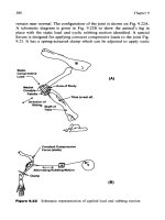
Hot water
inflow

Outflow
(a)

Energy exchange
Inflow
(from condensers)

Outflow

(to condensers)
(b)

FIGURE 5.47 The flow system for power plant heat rejection to a body of water: (a) Top
view, (b) front view.


Acceptable Design of a Thermal System

373

make up the overall system. Over the years, the power industry has developed
strategies to design and optimize such systems.
The design process is fundamentally the same for large and small systems
and the basic approach presented in this and earlier chapters can easily be applied
to a wide range of systems using the principles of modeling, simulation, design,
and optimization presented in this book. However, additional aspects pertaining
to safety, control, input/output, etc., need to be included in industrial systems
before the prototype is developed.

5.6 SUMMARY
This chapter presents the synthesis of various design steps needed to obtain
an acceptable design for a thermal system. Employing the basic considerations
involved in design, as outlined in the earlier chapters, an overview of the design
procedure is presented. Starting with the basic concept for the system, the various steps involved in design were given as formulation of the problem, initial
design, modeling, simulation, evaluation, iterative redesign, and convergence to
an acceptable design. Several of these aspects, particularly modeling and simulation, were presented in detail earlier and are applied in this chapter. Two ingredients in the design process that had not been discussed adequately earlier are
the development of an initial design and different design strategies. These are
presented in some detail in this chapter.
Initial design is an important element in the design process and is considered

in terms of the different methods that may be adopted to obtain a design that is as
close as possible to an acceptable design. A range of acceptable designs may be
obtained by changing the design variables, starting with the initial design values,
in the domain specified by the constraints. The development of an initial design
may be based on existing systems, selection of components to satisfy the requirements and constraints, use of a library of designs from previous efforts, and
current engineering practice for the specific application. In this way, the effort
exerted to obtain an appropriate initial design is considerably reduced by building
on available information and earlier efforts.
The main design strategy presented earlier was based on starting with an
initial design and proceeding with an iterative redesign process until a converged
acceptable design is obtained. This systematic approach is used quite extensively
in the design of thermal systems. However, several other strategies are possible
and are employed. In particular, extensive results on the system response to a variation in the design variables (for given operating conditions) as well as to different
operating conditions (for selected designs) may form the basis for obtaining an
acceptable design. Such strategies, though not as systematic as the previous one,
are nevertheless popular because extensive results can often be obtained easily
from numerical simulation. These strategies are also well suited to systems with
a small number of parts and those with only a few design variables. The methods
to track the iterative redesign process and to study the convergence characteristics
are also discussed.


374

Design and Optimization of Thermal Systems

In order to illustrate the coupling of the different aspects and steps involved
in the design process, several important areas of application are considered and a
few typical thermal systems that arise in these areas are considered as examples.
This discussion is important for understanding the design process because the

various steps involved in design had been discussed earlier as separate items. It
is important to understand how these are brought together for an actual thermal
system and how the overall process works.
Finally, this chapter presents additional considerations that are often important
in the design and successful implementation of a practical thermal system. Included
in this list are safety issues, control of the system, environmental effects, structural
integrity of the system, material selection, costs involved, availability of facilities,
governmental regulations, and legal issues. These considerations are important
and must usually be included in the final design. However, a detailed discussion
of these aspects is beyond the scope of this book. Several of these aspects are
included in the design process by a suitable choice of constraints for an acceptable
design. The application of this process to large practical systems is outlined.

REFERENCES
Avallone, E.A. and Baumeister, T., Eds. (1987) Marks’ Standard Handbook for Mechanical Engineers, 9th ed., McGraw-Hill, New York.
Bejan, A. (1993) Heat Transfer, Wiley, New York.
Bloch, H., Cameron, J., Danowski, F., James, R., Swearingen, J., and Weightman, M.
(1982) Compressors and Expanders, Marcel Dekker, New York.
Boehm, R.F. (1987) Design Analysis of Thermal Systems, Wiley, New York.
Brown, R. (1986) Compressors—Selection and Sizing, Gulf Publishing Company,
Houston, TX.
Cengel, Y.A. and Boles, M.A. (2002) Thermodynamics: An Engineering Approach, 4th
ed., McGraw-Hill, New York.
Fox, R.W. and McDonald, A.T. (2003) Introduction to Fluid Mechanics, 6th ed., Wiley,
New York.
Gebhart, B. (1971) Heat Transfer, 2nd ed., McGraw-Hill, New York.
Ghosh, A. and Mallik, A.K. (1986) Manufacturing Science, Ellis Horwood, Chichester,
U.K.
Gulf Publishing Company. (1979) Compressors Handbook for the Hydrocarbon Processing Industries, Gulf Publishing Company, Houston, TX.
Harvey, G.F. (1977) Mathematical simulation of tight coil annealing, J. Australasian Inst.

Metals, 22:28–37.
Howell, J.R. and Buckius, R.O. (1992) Fundamentals of Engineering Thermodynamics,
2nd ed., McGraw-Hill, New York.
Incropera, F.P. (1988) Convection heat transfer in electronic equipment cooling, ASME J.
Heat Transfer, 110:1097–1111.
Incropera, F.P. (1999) Liquid Cooling of Electronic Devices by Single-Phase Convection,
Wiley, New York.
Incropera, F.P. and Dewitt, D.P. (1990) Fundamentals of Heat and Mass Transfer, 3rd ed.,
Wiley, New York.
Incropera, F.P. and Dewitt, D.P. (2001) Fundamentals of Heat and Mass Transfer, 5th ed.,
Wiley, New York.


Acceptable Design of a Thermal System

375

Jaluria, Y. (1976) A study of transient heat transfer in long insulated wires, J. Heat
Transfer, 98:127–132, 678–680.
Jaluria, Y. (1984) Numerical study of the thermal processes in a furnace, Numerical Heat
Transfer, 7:211–224.
Janna, W.S. (1993) Design of Fluid Thermal Systems, PWS-Kent Publising Company,
Boston, MA.
Kakac, S., Shah, R.K., and Bergles, A.E., Eds. (1983) Low Reynolds Number Flow Heat
Exchangers, Taylor & Francis, Washington, DC.
Kalpakjian, S. and Schmid, S.R. (2005) Manufacturing Engineering and Technology, 5th
ed., Prentice-Hall, Upper Saddle River, NJ.
Kays. W.M. and London, A.L. (1984) Compact Heat Exchangers, 3rd ed., McGraw-Hill,
New York.
Kraus. A.D. and Bar-Cohen, A. (1983) Thermal Analysis and Control of Electronic Equipment, Hemisphere, Washington, DC.

Leinhard, J.H. (1987) A Heat Transfer Textbook, 2nd ed., Prentice-Hall, Englewood
Cliffs, NJ.
Moore, F.K. and Jaluria, Y. (1972) Thermal effects of power plants on lakes, ASME J.
Heat Transfer, 94:163–168.
Pollak, F., Ed. (1980) Pump Users’ Handbook, Gulf Publishing Company, Houston, TX.
Reynolds, W.C. and Perkins, H.C. (1977) Engineering Thermodynamics, 2nd ed.,
McGraw-Hill, New York.
Seraphin, D.P., Lasky, R.C., and Li, C.Y. (1989) Principles of Electronic Packaging,
McGraw-Hill, New York.
Shames, I.H. (1992) Mechanics of Fluids, 3rd ed., McGraw-Hill, New York.
Steinberg, D.S. (1980) Cooling Techniques for Electronic Equipment, Wiley-Interscience,
New York.
Stoecker, W.F. (1989) Design of Thermal Systems, 3rd ed., McGraw-Hill, New York.
Thompson, J.E. and Trickler, C.J. (1983) Fans and fan systems, Chem. Eng., March:46–63.
Van Wylen, G.J., Sonntag, R.E., and Borgnakke, C. (1994) Fundamentals of Classical
Thermodynamics, 4th ed., Wiley, New York.
Viswanath, R. and Jaluria, Y. (1991) Knowledge-based system for the computer aided
design of ingot casting processes, Eng. Comput., 7:109–120.
Warring, R. (1984) Pumps: Selection, Systems and Applications, 2nd ed., Gulf Publishing
Company, Houston, TX.

PROBLEMS
Note: Appropriate assumptions, approximations, and inputs may be employed to
solve the design problems in the following set. A unique solution is not obtained
for an acceptable design in many of these problems, and the range in which the
solution lies may be given wherever possible.
5.1. A refrigeration system is needed to provide 10 kW of cooling at 0 C,
with the ambient at 25 C. Obtain a workable or acceptable design to
achieve these requirements, assuming that a variation of 5 C in both
temperature levels is permissible. You may choose any appropriate

fluid, component efficiencies in the range 75 to 90%, and a suitable
thermodynamic cycle for the purpose.


376

Design and Optimization of Thermal Systems

5.2. Develop an acceptable design for a cooling system, using vapor compression, to achieve 0.5 ton of cooling at –10 C, with the ambient temperature as high as 40 C. The use of CFCs is not permitted because
of their environmental effect. The efficiency of the compressor may
be assumed to lie between 75 and 85%. Discuss any sensors that you
might need for temperature control.
5.3. A heat pump is to be designed to obtain a heat input of 2 kW into a region
that is at 25 C, as shown in Figure P5.3. The ambient temperature may be
as low as 0 C. Obtain an acceptable design to satisfy these requirements,
using efficiencies in the range 80 to 90% for the components. The only
constraint is that the working fluid should not undergo freezing.

25°C

2 kW
Heat pump

0°C
Ambient

Enclosed
space

FIGURE P5.3

5.4. For the casting process considered in Problem 3.7, briefly discuss the
simulation of the process and the anticipated results from the simulation. Develop a workable design for a thermal system to achieve the
desired heating.
5.5. In an oven, the support for the walls is provided by long horizontal
bars, of length L and square in cross-section, attached to two vertical
walls, as shown in Figure P5.5. A crossflow of ambient air, at velocity V and temperature Ta, cools the bars. The walls may be assumed
to be at uniform temperature Tw. We can vary Ta, the material of the
supporting bars, and the width H of the bars. The temperature at the
midpoint A, TA, must be less than a given value Tmax due to strength
considerations.
L
Tw

TA

H
A

x

V, Ta

FIGURE P5.5

H

Tw

H

Acceptable Design of a Thermal System

377

(a) Develop a suitable mathematical model for this system, giving the
governing equations and the relevant boundary conditions.
(b) Sketch the expected temperature distribution in the bar.
(c) What are the fixed quantities, requirements, and design variables
in the problem?
(d) Discuss the simulation of the system and obtain an acceptable
design for this application.
5.6. In the energy storage system consisting of concentric cylinders, considered in Problem 3.1, L and R2 are given as fixed, while R1 can be varied
over a given range, (R1)min R1 (R1)max. The approximations are the
same as those given before. The metal pieces are to be heated without
exceeding a maximum temperature Tmax and interest lies in storing the
maximum amount of energy.
(a) Formulate the corresponding design problem, focusing on quantities that can be varied.
(b) Simulate the system to determine the dependence of energy stored
on the design variables.
(c) Obtain an acceptable design.
5.7. If in the problem considered in Example 5.3, the hot water requirements are changed to 50 to 75 C, determine the effect on the final
results. Also, vary the ambient temperature to 30 C and determine the
range of acceptable designs.
5.8. A solar energy power system is to be designed to operate between 90 C,
at which hot water is available from the collectors, and 25 C, which is
the ambient temperature, in order to deliver 200 kW of power. Using
any appropriate fluid and thermodynamic cycle, obtain an acceptable
design for this process. Assume that boilers, compressors, and turbines

of efficiency in the range 70 to 80% are available for the purpose.
5.9. A cold storage room of inner dimensions 4 m 4 m 3 m and containing air is to be designed. The outside temperature varies from 40°C
during the day to 20°C at night. The outside heat transfer coefficient is
10 W/(m2 · K) and that at the inner surface of the wall is 20 W/(m2 · K).
A constant energy input of 4 kW may be assumed to enter the air
through the door, as shown in Figure P5.9. A refrigerator system is
used to extract energy from the enclosure floor. What are the important
design variables in this problem? Develop a simple model for simulating the system and obtain the refrigeration capacity needed. The
energy extracted by the refrigerator need not be constant with time.
Also, determine the values of the other design variables to maintain
a temperature of 5 C 2 C in the storage room. The wall thickness
must not exceed 15 cm, and it is desirable to have the smallest possible
refrigeration unit. Also, suggest any improvements that may be incorporated in your mathematical model for greater accuracy.


378

Design and Optimization of Thermal Systems

3m

4 kW

4m

4m

FIGURE P5.9

5.10. An electronic equipment is to be designed to obtain satisfactory cooling of the components. The available air space is 0.45 m 0.35 m

0.25 m. The distance between any two boards must be at least 5 cm.
The total number of components is 100, with each dissipating 20 W. The
dimensions of a board must not exceed 0.3 m 0.2 m. The heat transfer
coefficient may be taken as 20 W/(m2 · K) if there is only one board.
With each additional board, it decreases by 1 W/(m2 · K). Develop a suitable model for design of the system and obtain the minimum number of
boards needed to satisfy the temperature constraint of 100 C in an ambient at 20 C. How can your model be improved for greater accuracy?
5.11. In Example 5.4, the use of hollow mandrels is suggested as an improvement in the design. Consider this change and determine the effect on
the simulation and the design. However, the thickness of the wall of
the mandrel should not be less than 0.5 mm from strength considerations. Also, consider the circulation of hot fluid through the mandrel
to impose a higher temperature at the inner boundary of the plastic.
Determine the effect of this change on the design.
5.12. In the cooling system for electronic equipment considered in Example
5.5, determine the effect on the design of allowing the board height to
reach 0.2 m and of increasing the convective heat transfer coefficient
to 40 W/(m2 · K) by improving the cooling process. Consider the two
changes separately, taking the remaining variables as fixed. Discuss the
implications of these results with respect to the design of the system.
5.13. In a condenser, water enters at 20 C and leaves at temperature To. Steam
enters as saturated vapor at 90 C and leaves as condensate at the same
temperature, as shown in Figure P5.13. The surface area of the heat
exchanger is 2 m2 and a total of 250 kW of energy is to be transferred in
the heat exchanger. The overall heat transfer coefficient U is given by
U

m
0.05 0.2 m


Acceptable Design of a Thermal System

379

where m is the water mass flow rate in kg/s and U is in kW/(m2 · K).
Obtain the algebraic equation that gives the water flow rate m. Solve
this equation by the Newton-Raphson method, starting with an initial
guess between 0.5 and 0.9 kg/s. Also, calculate the outlet temperature To
for water. Take the specific heat and density of water as 4.2 kJ/(kg · K)
and 1000 kg/m3, respectively. What are the main assumptions made in
this model?
90°C
Steam
20°C
Water

To
Water
90°C
Condensate

FIGURE P5.13

5.14. In a counterflow heat exchanger, the cold fluid enters at 20 C and leaves
at 60 C. Its flow rate is 0.75 kg/s and the specific heat is 4.0 kJ/(kg · K).
The hot fluid enters at 80 C with a flow rate of 1.0 kg/s. Its specific heat
is 3.0 kJ/(kg · K). The overall heat transfer coefficient U is given as 200
W/(m2 · K). Calculate the outlet temperature of the hot fluid, the total
heat transfer Q, and the area A needed. What are the possible design
variables in this problem, if the cold fluid conditions are fixed?
5.15. In a counterflow heat exchanger, the cold fluid enters at 15 C. Its flow
rate is 1.0 kg/s and the specific heat is 3.5 kJ/(kg·K). The hot fluid enters

at 100 C at a flow rate of 1.5 kg/s. Its specific heat is 3.0 kJ/(kg · K).
The overall heat transfer coefficient U is given as 200 W/(m2 · K). It is
desired to heat the cold fluid to 60 5 C. Outline a simple mathematical model for this system, giving the main assumptions and approximations. What are the design variables in the problem? Calculate the
outlet temperature of the hot fluid, the total heat transfer q, and the area
A needed.
5.16. In a counterflow heat exchanger, cold water enters at 20 C and hot
water at 80 C, as shown in Figure P5.16. The two flow rates are
.
equal and denoted by m in kg/s. The specific heat is also given as the
same for the cold and hot water streams and equal to 3.0 kJ/(kg · K).
The value of the overall heat transfer coefficient U in kW/(m2 · K) is
given as
1
UA

0.1

0.2
m


380

Design and Optimization of Thermal Systems
Cold
Water
.
m
20°C

U

Hot
Water
.
m
80°C

FIGURE P5.16

5.17.

5.18.

5.19.

5.20.

where A is the surface area in square meters. Write down the relevant
mathematical model and, employing the Newton-Raphson method for
one equation, determine the value of m that results in a heat transfer
.
rate of 300 kW. Start with an initial guess of m between 3 and 3.5 kg/s.
Determine the sensitivity of the mass flow rate to the overall heat transfer rate by varying the latter about its given value of 300 kW.
Water at 40 C flows at m kg/s into a condenser that has steam condensing at a constant temperature of 110 C. The UA value of the heat
exchanger is given as 2.5 kW/K and the desired total heat transfer rate
is 120 kW. The specific heat at constant pressure Cp for water may be
taken as 4.2 kJ/(kg · K). Write the equation(s) to calculate m and, using any
simulation approach, determine the appropriate value of m for the given
heat transfer rate. If the total heat transfer rate varies as 120 20 kW,

determine the corresponding variation in m.
A heat exchanger is to be designed to heat water at 1.0 kg/s from 15 C
to 75 C. A parallel-flow heat exchanger is to be used and the hot fluid
is water at 100 C. Take the specific heat as 4200 J/(kg · K) for both
fluids. The mass flow rate of the hot fluid must not exceed 4 kg/s. The
diameter of the inner pipe must not exceed 0.1 m and the length of the
heat exchanger must be less than 100 m. Obtain an initial, acceptable
design for this process and give the dimensions of the heat exchanger.
Give a sketch of the temperature variation in the two fluid streams.
A condenser is to be designed to condense steam at 100 C to water at
the same temperature, while removing 300 kW of thermal energy. A
counterflow heat exchanger is to be employed. Water at 15 C is available for flow in the inner tube and the overall heat transfer coefficient
U is 2 kW/m2K. The temperature rise of the cooling water must not
be greater than 50 C, the inner tube diameter must not exceed 8 cm,
and the length of the heat exchanger must not exceed 20 m. Obtain an
acceptable design and give the corresponding mass flow rates, water
temperature at the exit, and heat exchanger dimensions.
Choose a design parameter Y to follow the convergence of iterative
redesign of a refrigeration system. Give reasons for your choice and
sketch its expected variation as the compressor is varied to change the
exit pressure.


Acceptable Design of a Thermal System

381

5.21. Decide on a design parameter Y to study the convergence of an iterative
design procedure for a shell and tube heat exchanger. If the design variables, such as tube and shell diameters, are varied to reach an acceptable design, how would you expect the chosen criterion Y to vary?
5.22. Take the refrigeration system considered in Example 5.1. If the storage facility is to be maintained in the temperature range of 0 to 5 C,

while the outside temperature range and the total thermal load remain
unchanged, redesign the system to achieve these requirements.
5.23. Develop the initial, acceptable design for the problem considered in
Example 5.2 if the maximum temperature obtainable from the heat
source is only 290 C.
5.24. Redesign the solar energy storage system considered in Example 5.3 if
the total amount of energy to be stored is halved, while the remaining
requirements remain the same. Also, choose a design parameter Y that
may be used to examine the convergence of the redesign process, giving reasons for your choice.
5.25. Redesign the heat exchanger considered in Example 5.7 for the requirements that the outer tube diameter be less than 6.0 cm and the inner
tube diameter be greater than 2.0 cm, keeping the remaining conditions unchanged.
5.26. Redesign the heat exchanger in Example 5.7 to obtain a total length of
less than 75.0 m, while keeping the outer tube diameter greater than 3.0
cm. No constraints are specified on the inner tube.
5.27. For a fluid flow system similar to the one considered in Example 5.8,
take the design values of P1, P2, H, A, B, and C as 470, 700, 135, 10,
20, and 5, respectively, in the units given earlier. Simulate this system,
employing the Newton-Raphson method. Study the effect on the total
flow rate of varying the zero-flow pressure values (470 and 700 in the
preceding equations) and the height (135) by 20%. Find the maximum
and minimum flow rates.
5.28. Determine the effect of varying the heat transfer coefficient to
100 W/(m2 · K) and the equilibrium temperature Te to 15 C in Example
5.6. Compare the results obtained with those presented earlier and discuss the implications for the design of a heat rejection system. What do
such changes mean in actual practice?
5.29. A plastic (PVC) plate of thickness 2 cm is to be formed in the shape of
an “N”. For this purpose, it must be raised to a uniform temperature of
200 C and held at this temperature for 15 sec to complete the process.
The temperature must not exceed the melting temperature, which is
300 C for this material. Develop a conceptual design and a mathematical model for this process. Obtain an acceptable design to achieve the

desired temperature variation.
5.30. The surface of a thick steel plate is to be heat treated to a depth of
2.5 mm. A constant heat flux input of 106 W/m2 is applied at the surface. The required temperature for heat treatment is 560 C, and the


382

Design and Optimization of Thermal Systems

maximum allowable temperature in the material is 900 C. Can this
arrangement be used to achieve an acceptable design? If so, determine
the time at which the heat input must be turned off. Can you suggest a
different or better design?
5.31. For the preceding problem, suggest a few conceptual designs and
choose one as the most appropriate. Justify your choice.


6

Economic Considerations

6.1 INTRODUCTION
Among the most important indicators of the success of an engineering enterprise
are the profit achieved and the return on investment. Therefore, economic considerations play a very important role in the decision-making processes that govern
the design of a system. It is generally not enough to make a system technically
feasible and to obtain the desired quality of the product. The costs incurred must
be taken into account to make the effort economically viable. It is necessary
to find a balance between the product quality and the cost, since the product
would not sell at an excessive price even if the quality were exceptional. For a
given item, there is obviously a limit on the price that the market will bear. As

discussed in Chapter 1, the sales volume decreases with an increase in the price.
Therefore, it is important to restrain the costs even if this means some sacrifice
in the product quality. However, in some applications, the quality is extremely
important and much higher costs are acceptable, as is the case, for instance, in
racing cars, rocket engines, satellites, and defense equipment. Similarly, a poorquality product at a low price is not acceptable. The key aspect here is finding a
proper balance between the quality and cost for a given application.
Even if it can be demonstrated that a project is technically sound and would
achieve the desired engineering goals, it may not be undertaken if the anticipated
profit is not satisfactory. Since most industrial efforts are directed at financial profit,
it is necessary to concentrate on projects that promise satisfactory return; otherwise,
investment in a given company would not be attractive. Similarly, a very large initial investment may make it difficult to raise the funds needed, and the project may
have to be abandoned. Decisions at various stages of the design are also affected by
economic considerations. The choice of materials and components, for instance, is
often guided by the costs involved. The use of copper, instead of gold and silver, in
electrical connections, despite the advantages of the latter in terms of corrosion resistance, is an example of such a consideration. The characteristics and production rate
of the manufactured item are also affected by the market demand and the associated
financial return. Thus, economic aspects are closely coupled with the technical considerations in the development of a thermal system to achieve the desired objectives.
Economic factors, though crucial in design and optimization, are not the only
nonengineering ingredients in decision making. As seen earlier, several additional
nontechnical aspects such as environmental, safety, legal, and political issues arise
and may influence the decisions made by industrial organizations. However, several
of these can be frequently considered as additional expenses and may again be cast
in economic terms. For instance, pollution control may involve additional facilities
383


384

Design and Optimization of Thermal Systems

to clean up the discharge from an industrial unit. The choice of forced draft cooling
towers over natural draft ones may be made because of local opposition to the latter due to undesirable appearance, resulting in greater expense. Even political and
legal concerns are often translated in terms of money and are included in the overall
costs. Indeed, litigation has been one of the major hurdles in the expansion of the
nuclear power industry. Providing transportation, housing, education, day-care, and
other facilities to workers satisfies important social needs, but these can again be
treated as economic issues because of the additional expenses incurred.
Because of the crucial importance of economic considerations in most engineering decisions, it is necessary to understand the basic principles of economics
and to apply these to the evaluation of investments, in terms of costs, returns,
and profits. An important concept that is fundamental to economic analysis is
the effect of time on the worth of money. The value of money increases as time
elapses due to interest added on to the principal amount. Therefore, if the same
amount of money is paid today or 10 years later, the two payments are not of
the same value. The payment today will be worth more 10 years later due to
interest and this dependence on time must be taken into account. Similarly, inflation reduces the value of money because prices go up with time, decreasing the
purchasing power of money. As we have often heard from our parents, what a
dollar could buy 50 years ago is many times more than what it can buy today.
Consequently, we generally consider economic aspects in terms of constant dollars at a given time, say 1980, in order to compare costs and returns. This involves
bringing all the payments, expenditures, and returns to a common point in time so
that the overall financial viability of an engineering enterprise can be evaluated.
This chapter first presents the basic principles involved in economic analysis,
particularly the calculation of interest, the consequent variation of the worth of
money with time, and the methods to shift different financial transactions to a
common time frame. Different forms of payment, such as lumped sum and series
of equal payments, and different methods of calculating interest that are used in
practice are discussed. Taxes, depreciation, inflation, and other important factors
that must generally be included in economic analysis are discussed. Thus, a brief
discussion of economic analysis is presented here in order to facilitate consideration of economic factors in design and optimization. For further details on
economic considerations, textbooks on the subject may be consulted. Some of the
relevant books are those by Riggs and West (1986), Collier and Ledbetter (1988),

Blank and Tarquin (1989), Thuesen and Fabrycky (1993), White et al. (2001),
Newnan et al. (2004), Park (2004), and Sullivan et al. (2005).
An important task in the design of systems is the evaluation of different
alternatives from a financial viewpoint. These alternatives may involve different
designs, locations, procurement of raw materials, strategies for processing, and so
on. Many of the important economic issues outlined in this chapter play a significant role in such evaluations. A few typical cases are included for illustration. The
importance of economic factors in the design of thermal systems is demonstrated.
The chapter also discusses the important issue of cost evaluation, considering different types of costs incurred in typical thermal systems.


Economic Considerations

385

6.2 CALCULATION OF INTEREST
A concept that is of crucial importance in any economic analysis is that of the
worth of money as a function of time. The value increases with time due to interest accumulated, making the same payment or loan at different times lead to different amounts at a common point in time. Similarly, inflation erodes the value
of money by reducing its buying capacity as time elapses. Both interest and inflation are important in analyzing and estimating costs, returns, and other financial
transactions. Let us first consider the effect of interest on the value of a lumped
sum, or given amount of money, as a function of time.

6.2.1 SIMPLE INTEREST
The rate of interest i is the amount added or charged per year to a unit in the local
currency, such as $1, of deposit or loan, respectively. Frequently, the interest rate
is given as a percentage, indicating the amount added per one hundred of the local
monetary unit. This is known as the nominal rate of interest, and it is usually a
function of time, varying with the economic climate and trends in the financial
market. The total amount of the loan or deposit is known as the principal. If the
interest is calculated only on the principal over a given duration, without considering the change in investment due to accumulation of interest with time and
without including the interest with the principal for subsequent calculations, the

resulting interest is known as simple interest. Then, the simple interest on the
principal sum P invested over n years is simply Pni, and the final amount F consisting of the principal and interest after n years is given by
F

P (1

ni)

(6.1)

Therefore, an investment of $1000 at 10% simple interest would yield $100 at the
end of each year. At the end of 5 years, the total amount becomes $1500. The
simple interest is very easy to calculate, but is seldom used because the interest
on the accumulated interest can be substantial. In addition, one could invest the
accumulated interest separately to draw additional interest. Therefore, interest on
the interest generated is usually included in the calculations, and this is known as
compound interest.

6.2.2 COMPOUND INTEREST
The interest may be calculated several times a year and then added to the amount
on which interest is computed in order to determine the interest over the next time
period. This procedure is known as compounding and is frequently carried out
monthly when the resulting amount, which includes the principal and the accumulated interest, is determined for calculating the interest over the next month. Compounding may also be done yearly, quarterly, daily, or at any other chosen frequency.
For yearly compounding, the sum F after one year is P(1 i), which becomes the
sum for calculating the interest over the second year. Therefore, the sum after two


386

Design and Optimization of Thermal Systems

years is P(1 i)2, after three years P(1 i)3, and so on. This implies that for yearly
compounding, the final sum F after n years is given by the expression
F

P (1

i)n

(6.2)

Clearly, a considerable difference can arise between simple and compound interest as the duration of the investment or loan increases and as the interest rate
increases. Figure 6.1 shows the resulting sum F for an investment of $100 as a
function of time at different interest rates, for both simple interest and annual
compounding of the interest. While simple interest yields a linear increase in F
with time, compound interest gives rise to a nonlinear variation, with the deviation from linear increasing as the interest rate or time increases. It is because of
the considerable difference that can arise between simple and compound interest
that the former is rarely used. In addition, different frequencies of compounding
are often employed to yield wide variations in interest.
If the interest is compounded m times a year, the interest on a unit amount in
the time between two compoundings is i/m. Then the final sum F, which includes
the principal and interest, is obtained after n years as
F

P 1

i
m

mn

(6.3)

Therefore, for a given lumped sum P, the final sum F after n years may be calculated
from Equation (6.3) for different frequencies of compounding over the year. Monthly
compounding, for which m 12, and daily compounding, for which m 365, are
very commonly used by financial institutions.

15%

F
800
700

Simple interest
Compound interest
Interest
rate =
10%

600
500
400

15%

300

10%
5%

5%

200

n

100
5

10

15

20

FIGURE 6.1 Variation of the sum F, consisting of the principal and accumulated interest,
as a function of the number of years n, for simple interest and for annual compounding at
different rates of interest.


Economic Considerations

387

It can be easily seen that a substantial difference in the accumulated interest arises for different compounding frequencies, particularly at large interest
rates. For instance, an investment of $1000 becomes $2000 after 10 years at a
simple interest of 10%, due to the accumulation of interest. The same investment
after the same duration becomes $2593.74 if yearly compounding is employed,
$2707.40 if monthly compounding is used, and $2717.91 if daily compounding is
used. Therefore, a higher compounding frequency leads to a faster growth of the

investment and is preferred when large financial transactions are involved.

6.2.3 CONTINUOUS COMPOUNDING
The number of times per year that the interest is compounded may be increased
beyond monthly or even daily compounding to reflect the financial status of a
company or an investment at a given instant. The upper limit on the frequency
of compounding is continuous compounding, which employs an infinite number
of compounding periods over the year. Thus, the interest is determined continuously as a function of time and the resulting sum at any given instant is employed
in calculating the interest for the next instant. Then the total amount at a given
instant is known, and investments and other financial transactions can be undertaken instantly based on the current financial situation.
As shown in the preceding section, the sum F after a period of n years with a
nominal interest rate of i compounded m times per year is given by Equation (6.3).
For continuous compounding, the frequency of compounding approaches infinity,
i.e., m
, which gives
F

P 1

i
m

mn

m

Therefore, taking the logarithm of both sides
ln

F

P

mn ln 1

i
m

mn
m

i
m

1 i
2 m

2

1 i
3 m

3

ni
m

where ln represents the natural logarithm. Here, ln(1 i/m) is expanded as a Taylor
series in terms of the variable i/m and m is allowed to approach infinity. Therefore,
from this equation, the sum F, for continuous compounding, is given by
F

Peni

(6.4)

If continuous compounding is used, an investment of $1000 for 10 years
would yield $2718.28, which is greater than the amounts obtained earlier with
other compounding frequencies. Continuous compounding is commonly used
in business transactions because the market varies from instant to instant and
monetary transactions occur continuously, making it necessary to consider the
instantaneous value of money in decision making.


388

Design and Optimization of Thermal Systems

6.2.4 EFFECTIVE INTEREST RATE
It is often convenient and useful to express the compounded interest in terms of
an effective, or equivalent, simple interest rate. This allows one to calculate the
resulting interest and to compare different investments more easily than by using
the compound interest formula, such as Equation (6.3). The effective interest rate
is also useful in analyzing economic transactions with different compounding
frequencies, as seen later. If ieff represents the effective simple interest for a given
compounding scheme, the sum F, which includes the principal and interest at the
end of the year, is simply
F

P (1

ieff )

(6.5)

Then ieff is obtained from Equation (6.3), for interest being compounded m times
per year, as
ieff

F
1
P

m

i
m

1

1
(6.6)

Similarly, for continuous compounding ieff ei – 1.
It is also possible to obtain an equivalent interest rate over a number of years n.
Then, from Equation (6.1),
F

P(1

nieff )

(6.7)

which gives

ieff

1 F
1
n P

1

i
m
n

mn

1
(6.8)

The effective interest rate, therefore, allows an easy calculation of the interest
obtained on a given investment, as well as that charged on a loan, making it simple to compare different financial alternatives. It is common for financial institutions to advertise the effective interest rate, or yield, paid over the duration of an
investment.
Example 6.1
Calculate the resulting sum F for an investment of $100 after 1, 2, 5, 10, 20, and
30 years at a nominal interest rate of 10%, using simple interest as well as yearly,
monthly, daily, and continuous compounding. From these results, calculate the
effective interest rates over a year and also 10 years.

Solution
The resulting sum F for a given investment P is obtained for simple interest, compounding m times yearly and for continuous compounding from the following three


Economic Considerations

389

TABLE 6.1
Effect of Compounding Frequency on the Resulting Sum for an Investment
of $100 after Different Time Periods at 10% Nominal Interest Rate
Number
of years

Simple
Interest

Yearly Comp.

Monthly Comp.

Daily Comp.

Continuous
Comp.

1

110.0

110.0

110.47

110.52

110.52

2

120.0

121.0

122.04

122.14

122.14

5

150.0

161.05

164.53

164.86

164.87

10

200.0

259.37

270.70

271.79

271.83

20

300.0

672.75

732.81

738.70

738.91

30

400.0

1744.94

1983.74

2007.73

2008.55

equations, respectively, given in the preceding sections:
F

P(1

F

P 1

F

ni)

Peni

i
m

mn

Therefore, the resulting sum F for an investment of $100 at a nominal interest rate of

10%, i.e., i 0.1, after a number of years n with different compounding frequencies,
may be calculated. The results obtained are shown in Table 6.1. It is obvious that large
differences in F arise over long periods of time, with continuous compounding yielding the largest amount. Simple interest, which considers the interest only on the initial
principal amount, yields a considerably smaller amount because interest on the accumulated interest is not taken into account. Consequently, simple interest is not appropriate for most financial transactions and is generally not used. In addition, the difference
between continuous and daily compounding is small. However, even this effect can be
quite significant if large investments, expenditures, and payments are involved.
The effective interest rate ieff is given by the equation
ieff

F
1
P

Therefore, ieff may easily be obtained from Table 6.1 by using the calculated values
of F after one year for the given investment of $100. It is seen that ieff is equal to
the nominal interest rate i 0.1 for simple interest and for yearly compounding, as
expected. For monthly, daily, and continuous compounding, ieff is 0.1047, 0.1052,
and 0.1052 (10.47, 10.52, and 10.52%), respectively.
The effective interest rates for yearly, monthly, daily, and continuous compounding over a period of 10 years may similarly be calculated using the equation
ieff

1 F
1
n P


390

Design and Optimization of Thermal Systems

Using the values given in Table 6.1, the effective interest rates for yearly, monthly,
daily, and continuous compounding are obtained as 15.937, 17.070, 17.179, and
17.183%, respectively, which are much higher than the nominal interest rate of 10%.
These effective rates may be used to calculate the interest or sum after 10 years
from Equation (6.7) with n 10.

6.3 WORTH OF MONEY AS A FUNCTION OF TIME
It is seen from the preceding discussion that the value of money is a function
of time. In order to compare or combine amounts at different times, it is necessary to bring these all to a common point in time. Once various financial
transactions are obtained at a chosen time, it is possible to compare different
financial alternatives and opportunities in order to make decisions on the best
course of action. Different costs, over the expected duration of a project, and
the anticipated returns can then be considered to determine the rate of return
on the investment and the economic viability of the enterprise. Two approaches
that are commonly used for bringing all financial transactions to a common
time frame are the present and future worth of an investment, expenditure, or
payment.

6.3.1 PRESENT WORTH
As the name suggests, the present worth (PW) of a lumped amount given at a particular time in the future is its value today. Thus, it is the amount that, if invested
at the prevailing interest rate, would yield the given sum at the future date. Let us
consider Equation (6.2), which gives the resulting sum F after n years at a nominal interest rate i. Then P is the present worth of sum F for the given duration and
interest rate. Therefore, the present worth of a given sum F may be written, for
yearly compounding, as
PW

P

F(1

i)

n

(F)(P/F, i, n)

(6.9a)

where P/F is known as the present worth factor and is given by
P/F

(1

i)

n

(6.9b)

This notation follows the scheme used in many textbooks on engineering economics; see, for example, Collier and Ledbetter (1988). Here, the applicable interest rate i and the number of years n are included in the parentheses along with the
present worth factor.
If the interest is compounded m times yearly, Equation (6.3) may be used to
obtain the present worth as
PW

P

( F ) P/F ,

i

, mn
m

(6.10a)


Economic Considerations

391

where the present worth factor P/F is given by
P/F

1
i
1
m

1

mn

i
m

mn

(6.10b)

Similarly, for continuous compounding

P/F

e

ni

(6.11)

Therefore, the present worth factor P/F may be defined and calculated for
different frequencies of compounding. The present worth of a given lumped
amount F representing a financial transaction, such as a payment, income, or
cost, at a specified time in the future may then be obtained from the preceding
equations.
The present worth of the resulting sums shown in Table 6.1 for different
duration and frequency of compounding is $100. Therefore, the present worth of
$1983.74 after 30 years with monthly compounding at 10% interest is $100, since
the latter amount will yield the former if it is appropriately invested. In design, a
specific amount in the future is commonly given and its present worth is determined using the applicable interest rate and compounding frequency. An example
of such a calculation is the expected expenditure on maintenance of an industrial
facility at a given time in the future. This financial transaction is then put in terms
of the present in order to consider it along with other expenses.
The concept of present worth is useful in evaluating different financial alternatives because it allows all transactions to be considered at a common time
frame. It also makes it possible to estimate the expenses associated with a given
system, financial outlay needed, and return on the investment, all usually based
on the expected duration of the project. Financial considerations are important
in decision making at various stages of the design and optimization process, for
instance during selection of materials and components. These decisions require
that all financial dealings be brought to a specified point in time, and the present
worth of different transactions is commonly used for this purpose. For instance,
at the end of useful life of the system, it will be disposed or sold. This expense or

financial gain is in the future and, therefore, it is usually brought to the present
time frame, using the concept of present worth, to include its effect in the overall
financial considerations of the system. It is also possible to base such financial
considerations on a point of time in the future, for which the concept of future
worth, outlined in the following section, is used.

6.3.2 FUTURE WORTH
The future worth of a lumped amount P, given at the present time, may similarly
be determined after a specified period of time. Therefore, the future worth (FW)
of P after n years with an interest rate of i, compounded yearly or m times yearly,


392

Design and Optimization of Thermal Systems

are given, respectively, by the following equations:
FW
FW

F

F

P (1

P 1

i
m

i)n

(P)(F/P, i, n)

mn

( P ) F / P,

(6.12a)

i
, mn
m

(6.12b)

where F/P is known as the future factor worth or compound amount factor. For
continuous compounding, F/P eni. Therefore, the future worth of a given lumped
sum today may be calculated at a specified time in the future if the compounding
conditions and the interest rate are given.
Again, the future worth of $100 after different time periods and with different
compounding frequencies, at a 10% nominal interest rate, may be obtained from
Table 6.1. Using these results, the future worth of $1200 after 10 years of daily
compounding at 10% interest is 12 271.79 $3261.48. Similarly, the future
worth for other lumped sums may be calculated for specified future date, interest
rate, and compounding. Table 6.2 shows the effect of interest rate on the future
worth with monthly compounding. As expected, the effect increases as the duration increases, resulting in almost a 20-fold difference between the future worths
for 5% and 15% after 30 years.
As with present worth, the concept of future worth may be employed to bring

all the relevant financial transactions to a common point in time. Frequently, the
chosen time is the end of the design life of the given system. Therefore, if a telephone switching system is designed to last for 15 years, the end of this duration
may be chosen as the point at which all financial dealings are considered. Once
the net profit or expenditure is determined, it can be easily moved to the present,
if desired. The financial evaluation of a given design or system is independent of
the time frame chosen for the calculations. Whether the present or the future time
is employed is governed largely by convenience and by the time at which data are
available. Clearly, if most of the data are available at the early stages of the project,

TABLE 6.2
Effect of Interest Rate on the Future Worth of $100
with Monthly Compounding
Interest Rate
Number of Years
5
10
15
20
25
30

5%

8%

10 %

12 %

15 %

128.36
164.71
211.37
271.26
348.13
446.77

148.98
221.96
330.69
492.68
734.02
1093.57

164.53
270.70
445.39
732.81
1205.69
1983.74

181.67
330.04
599.58
1089.26
1978.85
3594.96

210.72

444.02
935.63
1971.55
4154.41
8754.10


Economic Considerations

393

it is better to use present worth since the interest rates are better known close to
the present. In addition, the duration of a given enterprise may not be specified or
a definite time in the future may not clearly indicated, making it necessary to use
the present worth as the basis for financial analysis and evaluation.
Example 6.2
The design of the cooling system for a personal computer requires a fan. Three different manufacturers are willing to provide a fan with the given specifications. The first
one, Fan A, is at $54, payable immediately on delivery. The second one, Fan B, requires
two payments of $30 each at the end of the first and second years after delivery. The
last one, Fan C, requires a payment of $65 at the end of two years after delivery. Since
a large number of fans are to be purchased, the price is an important consideration.
Consider three different interest rates, 6, 8, and 10%. Which fan is the best buy?

Solution
In order to compare the costs of the three fans, the expenditure must be brought to
a common time frame. Choosing the time of delivery for this purpose, the present
worth of the expenditures on the three fans must be calculated. The cost of Fan A
is given at delivery and, therefore, its present worth is $54. For the other two fans,
the present worth at an interest rate of 6% are
Fan B:

PW

(30)(P/F, 6%, 1)
30
(1 0.06)

Fan C:

PW

(65)(P/F, 6%, 2)

(30)(P/F, 6%, 2)

30
(1 0.06)2
65
(1 0.06)2

28.30

26.70

$55.00

$57.85

Therefore, Fan A is the cheapest one at this interest rate.
At 8% interest rate, a similar calculation yields the present worth of the cost for

Fan B as $53.50 and that for Fan C as $55.73. Therefore, Fan B is the cheapest one
at this rate. At 10% interest rate, the corresponding values are $52.07 for Fan B and
$53.72 for Fan C. Again, Fan B is the cheapest, but even Fan C becomes cheaper
than Fan A. This example illustrates the use of present worth to choose between
different alternatives for system design.

6.3.3 INFLATION
Inflation refers to the decline in the purchasing power of money with time due
to increase in the price of goods and services. This implies that the return on an
investment must be considered along with the inflation rate in order to determine
the real return in terms of buying power. Similarly, labor, maintenance, energy,
and other costs increase with time and this increase must be considered in the
economic analysis of an engineering enterprise. For example, if the wages of a
given worker increase from $10 per hour to $11 per hour, while the price of a loaf
of bread goes from $1 to $1.10, the worker can still buy the same amount of bread


394

Design and Optimization of Thermal Systems

and does not see a real increase in income. In order to obtain a real increase in
income, the pay increase must be greater than the inflation rate. Thus, the buying
power of a person may increase or decrease with time, depending on the rate
of increase in income and the inflation rate. For industrial investments, it is not
enough to have a rate of return that keeps pace with the inflation. The return must
be higher to make a project financially attractive.
Inflation is often obtained from the price trends for groups of items that are
of particular interest to a given industry or section of society. The most common
measure of prices is the Consumer Price Index (CPI), obtained by the U.S. Department of Labor by tracking the prices of about 400 different goods and services.

The current base year is 1983, at which point the CPI is assigned a value of 100.
Table 6.3 gives the CPI from 1983 to 2005, along with the percent change from the
previous year. The CPI is frequently used as a measure of the inflation rate. Note
that the increase rate fluctuates from year to year. It represents the general trends in
inflation, not the specific change for a particular situation or application. Similarly,
other cost measures, such as the Construction Cost Index and the Building Cost
Index, representing cost of construction in terms of materials and labor, respectively, are employed to determine the inflation rate for the construction industry.
The large inflation rates in the late 1970s and early 1980s significantly hampered
the growth of the economy and have decreased to about 3% in recent years.
If the inflation rate is denoted by j, then the interest rate i must be equal to j
for the buying power to remain unchanged, i.e., the future worth F of a principal
amount P must equal P(1 j)n. If i > j, there is an increase in the buying power.
Denoting this real increase in buying power by ir, we may write by equating
future worth amounts,
F

P (1

i)n

P (1

j)n (1

ir )n

(6.13)

TABLE 6.3
Consumer Price Index (CPI)

Year

CPI

Percent Change

Year

CPI

Percent Change

1983
1984
1985
1986
1987
1988
1989
1990
1991
1992
1993

100
103.9
107.6
109.6
113.6
118.3

124.0
130.7
136.2
140.3
144.5

3.8
3.9
3.8
1.1
4.4
4.4
4.6
6.1
3.1
2.9
2.7

1994
1995
1996
1997
1998
1999
2000
2001
2002
2003
2004

148.2
152.4
156.9
160.5
163.0
166.6
172.2
177.1
179.9
184.0
188.9

2.7
2.5
3.3
1.7
1.6
2.7
3.4
1.6
2.4
1.9
3.3

2005
Source: Monthly Labor Review, U.S. Dept. of Labor

195.3

3.4

Economic Considerations

395

Therefore,
ir

1 i
1 j

1

(6.14)

This implies that, as expected, ir i if j 0, ir 0 if i j, and ir is positive for
i > j. From this equation, we can also calculate the interest rate i needed to yield
a desired real rate of increase in purchasing power, for a given inflation rate, as
i (1 j) (1 ir) – 1. For example, if the inflation rate is 5% and the interest
rate is 10%, the real interest rate, which gives the increase in the buying power, is
(1.1/1.05) – 1 0.0476, or 4.76%. Similarly, if an 8% real return is desired with the
same inflation rate, the interest rate needed is (1.05)(1.08) – 1 0.134 or 13.4%.
Different compounding frequencies may also be considered by replacing (1 i)n
in Equation (6.13) by (1 i/m)mn or by employing the effective interest rate, as
illustrated in the following example.
Example 6.3
An engineering firm has to decide whether it should withdraw an investment that
pays 8% interest, compounded monthly, and use it on a new product. It would
undertake the new product if the real rate of increase in buying power from the

current investment is less than 4%. The rate of inflation is given as 3.5%. Calculate
the real rate of increase in buying power. Will the company decide to go for the new
product? What should the yield from the investment be if the company wants a 5%
rate of increase in buying power?

Solution
The real rate of increase in buying power ir is given by the equation
ir

1 ieff
1 j

1

where j is the inflation rate and the effective interest rate ieff is given by
ieff

1

i
m

m

1

Here, the nominal interest rate is given as 8%. Therefore, for monthly compounding,
ieff

1

0.08
12

12

1 0.083

This gives the value of ir as
ir

1.083
1.035

1

0.0464


396

Design and Optimization of Thermal Systems

Therefore, the real increase in purchasing power from the present investment is
4.64%. Since this is not less than 4%, the firm will continue this investment and
not undertake development of the new product. However, if the inflation rate were
to increase, the real rate will decrease and the company may decide to go for the
new product.
To obtain a 5% real rate of increase in buying power from the current investment, the effective interest rate ieff is governed by the equation
ieff

ir)(1

j)

1

(1.05)(1.035)

1

0.087

(1

which gives
ieff

The nominal interest rate i may be obtained from the relationship between i and
ieff, given above, as
i

ieff )1/12

12[(1

12 (1.0871/12

1]

1)

0.0835

Therefore, a nominal interest rate of 8.35%, compounded monthly, is needed from
the current investment to yield a real rate of increase in buying power of 5%.

6.4 SERIES OF PAYMENTS
A common circumstance encountered in engineering enterprises is that of a series
of payments. Frequently, a loan is taken out to acquire a given facility and then
this loan is paid off in fixed payments over the duration of the loan. Recurring
expenses for maintenance and labor may be treated similarly as a series of payments over the life of the project. Both fixed and varying amounts of payments
are important, the latter frequently being the result of inflation, which gives rise
to increasing costs. The series of payments is also brought to a given point in time
for consideration with other financial aspects. As before, the time chosen may be
the present or a time in the future.

6.4.1 FUTURE WORTH OF UNIFORM SERIES OF AMOUNTS
Let us consider a series of payments, each of amount S, paid at the end of each
year starting with the end of the first year, as shown in Figure 6.2. The future
worth of this series at the end of n years is to be determined. This can be done
easily by summing up the future worths of all these individual payments. The first
payment accumulates interest for n – 1 years, the second for n – 2 years, and so
on, with the second-to-last payment accumulating interest for 1 year and the last
payment accumulating no interest. Therefore, if i is the nominal interest rate and
yearly compounding is used, the future worth F of the series of payments is given
by the expression
F

S[(1

i)n

1

(1

i)n

2

(1

i)n

3

(1

i)

1]

(6.15)