Design and Optimization of Thermal Systems Episode 2 Part 9 pps
Bạn đang xem bản rút gọn của tài liệu. Xem và tải ngay bản đầy đủ của tài liệu tại đây (216.54 KB, 25 trang )
422
Design and Optimization of Thermal Systems
Dieter, G.E. (2000) Engineering Design, 3rd ed., McGraw-Hill, New York.
Newnan, D.G., Eschenbach, T.G., and Lavelle, J.P. (2004) Engineering Economic Analysis,
9th ed., Oxford University Press, Oxford, U.K.
Park, C.S. (2004) Fundamentals of Engineering Economics, Prentice-Hall, Upper Saddle
River, NJ.
Riggs, J.L. and West, T. (1986) Engineering Economics, 3rd ed., McGraw-Hill, New York.
Stoecker, W.F. (1989) Design of Thermal Systems, 3rd ed., McGraw-Hill, New York.
Sullivan, W.G., Wicks, E.M., and Luxhoj, J. (2005) Engineering Economy, 13th ed.,
Prentice-Hall, Upper Saddle River, NJ.
Thuesen, G.J. and Fabrycky, W.J. (1993) Engineering Economy, 8th ed., Prentice-Hall,
Englewood Cliffs, NJ.
White, J.A., Agee, M.H., and Case, K.E. (2001) Principles of Engineering Economic
Analysis, 4th ed., Wiley, New York.
PROBLEMS
6.1. A steel plant has a hot-rolling facility for steel sheets that is to be sold
to a smaller company at $15,000 after 10 years. What is the present
worth of this salvage price if the interest is 8%, compounded annually? Also, calculate the present worth for an interest rate of 12% with
annual compounding. Will the present worth be larger or smaller if
the compounding frequency was increased to monthly? Explain the
observed behavior.
6.2. A chemical company wants to replace its hot water heating and storage
system. One buyer offers $10,000 for the old system, payable immediately on delivery. Another buyer offers $15,000, which is to be paid five
years after delivery of the old system. If the current interest rate is 10%,
compounded monthly, which offer is better financially?
6.3. A company wants to put aside $150,000 to meet its expenditure on repair
and maintenance of equipment. Considering yearly, quarterly, monthly,
and daily compounding, determine the total annual interest the company
will get in these cases if the nominal interest rate is 7.5%.
6.4. For nominal interest rates of 8 and 12%, calculate the effective interest
rates for yearly, quarterly, monthly, daily, and continuous compounding.
6.5. A company acquires a manufacturing facility by borrowing $750,000
at 8% nominal interest, compounded daily. The loan has to be paid off
in 10 years with payments starting at the end of the first year. Calculate the effective annual rate of interest and the amount of the annual
payment.
6.6. In the preceding problem, calculate the amount of the loan left after
four and after eight payments. Also, calculate the total amount of interest paid by the company over the duration of the loan.
6.7. A food processing company wants to buy a facility that costs $500,000.
It can obtain a loan for 10 years at 10% interest or for 15 years at 15%
interest. In both cases, yearly payments are to be made starting at the
end of the first year.
Economic Considerations
423
(a) Which alternative has a lower yearly payment?
(b) What is the loan amount paid off after 5 years for the two cases?
What are the amounts needed to pay off the entire loan at this time?
6.8. A company makes a profit of 10%. Calculate the real profit in terms of
buying power for inflation rates of 4, 6, and 8%.
6.9. A firm wants to have an actual profit of 8% in terms of buying power.
If the inflation rate is 11%, calculate the profit that must be achieved by
the firm in order to achieve its goal.
6.10. A small chemical company wants to obtain a loan of $120,000 to buy a
plastic recycling machine. It has the option of a loan at 6% interest for
10 years or a loan at 8% for 8 years, with monthly compounding and
payment in both the cases. Calculate the monthly payments in the two
cases, assuming that the first payment is made at the end of the first
month. Also, calculate the total interest paid in the two options.
6.11. A $1000 bond has 4 years to maturity and pays 8% interest twice a
year. If the current interest is 6% compounded annually, calculate the
sale price of the bond. Repeat the problem if the current interest is
compounded daily.
6.12. A $5000 bond has 5 years to maturity and it pays 7% interest at the end of
each year. If it is sold at $4500, calculate the current nominal interest.
6.13. A pharmaceutical company wants to acquire a packaging machine. It can
buy it at the current price of $100,000 or rent it at $18,000 per year. The
rental payments are to be made at the beginning of each year, starting on
the date the machine is delivered. If the interest rate is 10%, compounded
annually, and if the machine becomes the property of the company after
10 yearly payments, which option is better economically?
6.14. In the preceding problem, if the machine has a salvage value of $15,000
at the end of 10 years for the option of buying the facility, will the conclusions change? If the rate is 20%, with salvage, how will the results
change?
6.15. An industrial concern wants to procure a manufacturing facility. It can
buy an old machine by paying $50,000 now and 10 yearly payments of
$2,000 each, starting at the end of the first year. It can also buy a new
machine by paying $100,000 now and 5 yearly payments of $1000
each, starting at the end of the sixth year. The salvage value is $10,000
and $20,000 in the two cases, respectively. The nominal interest rate is
10%. Which is the better option, assuming that the performance of the
two machines is the same?
6.16. As a project engineer involved in the design of a manufacturing facility, you need to acquire a polymer injection-molding machine. Two
options are available from two different companies. The first one,
option A, requires 15 payments of $8000 per year, paid at the beginning of each year and starting immediately. The second one, option B,
requires eight payments of $15,000 per year, paid at the end of each
424
6.17.
6.18.
6.19.
6.20.
6.21.
6.22.
Design and Optimization of Thermal Systems
year and starting at the end of the first year. Determine which option
is better economically if the interest rate is 8%. Also, calculate the
amounts needed to pay off the loan after half the number of payments
have been made in the two options.
A company needs 1000 thermostats a year for a factory that manufactures heating equipment. It can buy these at $10 each from a subcontractor, with payment made at the beginning of each year for the annual
demand. It can also procure a facility at $75,000, with $2000 needed
for maintenance at the end of each year, to manufacture these. If the
facility has a life of 10 years and a salvage value of $10,000 at the end
of its life, which option is more economical? Take the interest rate as
8% compounded annually.
In the preceding problem, calculate the annual demand for thermostats
at which the two options will incur the same expense.
You have designed a thermal system that needs a plastic part in the
assembly. You can either buy the required number of parts from a manufacturer or buy an injection-molding machine to produce these items
yourself. The number of items needed is 2000 every year. In the first
option, you have to pay $12 per item for the yearly consumption at the
beginning of each year. The chosen life of the project is 10 years. For
the other option, you can lease a machine for $20,000 each year, paid
at the end of each year for 10 years. The maintenance of the machine
and raw materials cost $1000 at the end of the first year, $2000 at
the end of the second year, and increasing by $1000 each year, until
the last payment of $9000 is made at the end of the ninth year. Provide the payment schedule for the second option and determine which
option is better financially. Take the interest rate as 10%, compounded
annually.
A manufacturer of electronic equipment needs 10,000 cooling fans
over a year. The company can buy these for $20 each, payable on delivery at the beginning of each year, or at $24, payable two years after
delivery. Which is the better financial alternative if the interest rate is
9% compounded daily? Also, calculate the results if the interest rate
drops to 8%.
A gas burner needed for a furnace can be purchased from three different suppliers. The first one wants $100 for each burner, payable on
delivery. The second supplier is willing to take payments of $55 each
at the end of six months and the year. The third supplier claims that
his deal is the best and asks for $110 at the end of the year. The current
interest rate is 8.5%, compounded continuously. Since a large number
of burners are to be bought, it is important to get the best financial deal.
Whom would you recommend? Would your recommendation change if
the interest rate were to go up, say to 12%?
A company acquires a manufacturing facility for $300,000, to be paid in
15 equal annual payments starting at the end of the first year. The rate of
Economic Considerations
425
interest is 8%, compounded annually. After six payments, the company
is in good financial condition and wants to pay off the loan in four more
equal annual payments, starting with the end of the seventh year, as
shown in Figure P6.22. Calculate the first and the last payment (at the
end of the tenth year) made by the company.
1
2
3
4
5
6
7
8
9
10
Years
$300,000
FIGURE P6.22
6.23. An industry takes a loan of $200,000 for a machine, to be paid off in
10 years by annual payments beginning at the end of the first year.
The rate of interest is 10%, compounded monthly. At the end of five
payments, the company finds itself in a good financial situation and
management decides to pay off the loan in the following year, as shown
in Figure P6.23. How much does it have to pay at the end of the sixth
year to end the debt? Also, calculate the amount of the annual payment
in the first 5 years.
Final
payment
1
2
3
4
5
6
Years
$200,000
FIGURE P6.23
6.24. A company is planning to buy a machine, which requires a down payment of $150,000 and has a salvage value of $30,000 after 10 years.
The cost of maintenance is covered by the manufacturer up to the end
of 3 years. For the fourth year, the maintenance cost is $1000, paid
at the end of the year. These costs increase by $1000 each year until
the end of the tenth year, when the company pays for the maintenance
of the facility and sells it, as shown in Figure P6.24. The rate of interest is 10%, compounded annually. Find the present worth of buying
426
Design and Optimization of Thermal Systems
and maintaining the machine over 10 years. If the company wants to
take out a fixed amount annually from its income to cover the entire
expense, calculate this amount, starting at the end of the first year.
Years
1
2
3
4
5
6
7
8
9
10
$30,000
Salvage
$150,000
Down payment
FIGURE P6.24
6.25. A manufacturing company wants to buy a welding machine, which
costs $10,000. The cost of maintenance is zero in the first year, $500
in the second year, and increases by $500 each year until the eighth
year when the company pays the maintenance expense and sells the
facility for $2000. The maintenance expense is paid at the end of each
year. The rate of interest is 9%, compounded annually. Find the present
worth of acquiring and maintaining this machine over 8 years.
6.26. A company is considering the purchase and operation of a manufacturing system. The initial cost of the system is $200,000 and the maintenance costs are zero at the end of the first year, $5000 at the end of
the second year, $10,000 at the end of the third year, and continue to
increase by $5000 each year. If the life of the system is 15 years, find
the present worth of buying and maintaining it over this period. Also,
find the uniform annual amount that the system costs the company
each year, starting after the first year. Take the interest rate as 10%
compounded annually.
6.27. An industrial firm wants to acquire a laser-cutting machine. It can buy
a new one by paying $150,000 now and six yearly payments of $20,000
each, starting at the end of the fifth year. It can also buy an old machine by
paying $100,000 now and 10 yearly payments of $15,000, starting at the
end of the first year. At the end of 10 years, the salvage value of the new
machine is $80,000 and that of the old one is $60,000. Which is the better
purchase for the firm, if the interest rate is 12% compounded annually?
Use lifecycle savings. Repeat the calculation for a 10% interest rate.
6.28. Using the data given in Example 6.7, choose between the two machines
for interest rates of 4, 6, and 10%. Compare the results obtained with
Economic Considerations
427
those given in the example and discuss the implications of the observed
trends.
6.29. Again using the data given in Example 6.7, study the effects of the useful
lives of the machines on their economic viability. Consider useful life
durations of 4, 8, and 10 years. Discuss the implications of the results
obtained in making appropriate choices in the design process based on
costs.
6.30. Calculate the rates of return for the two facilities given in Example 6.8
as functions of the useful lives of the facilities. Take the life as 4, 6, and
8 years, and calculate the corresponding rates of return with and without taxes at the rate of 50% of the profit taken into account. Compare
these with the earlier results and comment on their significance in the
design process.
6.31. A loan of $5000 is taken from a bank that charges a nominal interest
rate i, compounded monthly. If a monthly payment of $200, starting at
the end of the first month, is needed for 36 months to pay off the loan,
calculate the value of i.
7
Problem Formulation
for Optimization
7.1 INTRODUCTION
In the preceding chapters, we focused our attention on obtaining a workable, feasible,
or acceptable design of a system. Such a design satisfies the requirements for the
given application, without violating any imposed constraints. A system fabricated
or assembled because of this design is expected to perform the appropriate tasks for
which the effort was undertaken. However, the design would generally not be the
best design, where the definition of best is based on cost, performance, efficiency,
or some other such measure. In actual practice, we are usually interested in obtaining the best quality or performance per unit cost, with acceptable environmental
effects. This brings in the concept of optimization, which minimizes or maximizes
quantities and characteristics of particular interest to a given application.
Optimization is by no means a new concept. In our daily lives, we attempt
to optimize by seeking to obtain the largest amount of goods or output per unit
expenditure, this being the main idea behind clearance sales and competition. In
the academic world, most students try to achieve the best grades with the least
amount of work, hopefully without violating the constraints imposed by ethics
and regulations. The value of various items, including consumer products like
televisions, automobiles, cameras, vacation trips, advertisements, and even education, per dollar spent, is often quoted to indicate the cost effectiveness of these
items. Different measures of quality, such as durability, finish, dependability,
corrosion resistance, strength, and speed, are included in these considerations,
often based on actual consumer inputs, as is the case with publications such as
Consumer Reports. Thus, a buyer, who may be a student (or a parent) seeking an
appropriate college for higher education, a couple looking for a cruise, or a young
professional searching for his first dream car may use information available on
the best value for their money to make their choice.
7.1.1
OPTIMIZATION IN DESIGN
The need to optimize is similarly very important in design and has become particularly crucial in recent times due to growing global competition. It is no longer
enough to obtain a workable system that performs the desired tasks and meets the
given constraints. At the very least, several workable designs should be generated
and the final design, which minimizes or maximizes an appropriately chosen
quantity, selected from these. In general, many parameters affect the performance
and cost of a system. Therefore, if the parameters are varied, an optimum can
429
430
Design and Optimization of Thermal Systems
often be obtained in quantities such as power per unit fuel input, cost, efficiency,
energy consumption per unit output, and other features of the system. Different
product characteristics may be of particular interest in different applications and
the most important and relevant ones may be employed for optimization. For
instance, weight is particularly important in aerospace and aeronautical applications, acceleration in automobiles, energy consumption in refrigerators, and flow
rate in a water pumping system. Thus, these characteristics may be chosen for
minimization or maximization.
Workable designs are obtained over the allowable ranges of the design variables in order to satisfy the given requirements and constraints. A unique solution is generally not obtained and different system designs may be generated for
a given application. We may call the region over which acceptable designs are
obtained the domain of workable designs, given in terms of the physical variables
in the problem. Figure 7.1 shows, qualitatively, a sketch of such a domain in terms
of variables x1 and x2, where these may be physical quantities such as the diameter
and length of the shell in a shell-and-tube heat exchanger. Then, any design in this
domain is an acceptable or workable design and may be selected for the problem
at hand. Optimization, on the other hand, tries to find the best solution, one that
minimizes or maximizes a feature or quantity of particular interest in the application under consideration. Local extrema may be present at different points in
the domain of acceptable designs. However, only one global optimal point, which
yields the minimum or maximum in the entire domain, is found to arise in most
applications, as sketched in the figure. It is this optimal design that is sought in
the optimization process.
x1
Optimum
design
Domain of
acceptable
designs
x2
FIGURE 7.1 The optimum design in a domain of acceptable designs.
Problem Formulation for Optimization
7.1.2
431
FINAL OPTIMIZED DESIGN
The optimization process is expected to yield an optimal design or a subdomain
in which the optimum lies, and the final system design is obtained on the basis
of this solution. The design variables are generally not taken as exactly equal
to those obtained from the optimal solution, but are changed somewhat to use
more convenient sizes, dimensions, and standard items available in the market.
For instance, an optimal dimension of 4.65 m may be taken as 5.0 m, a 8.34 kW
motor as a 10 kW motor, or a 1.8 kW heater as a 2.0 kW heater, because items with
these specifications may be readily available, rather than having the exact values
custom made. An important concept that is used at this stage to finalize the design
variables is sensitivity, which indicates the effect of changing a given variable on
the output or performance of the system. In addition, safety factors are employed
to account for inaccuracies and uncertainties in the modeling, simulation, and
design, as well as for fluctuations in operating conditions and other unforeseen
circumstances. Some changes may also be made due to fabrication or material
limitations. Based on all these considerations, the final system design is obtained
and communicated to various interested parties, particularly those involved in
fabrication and prototype development.
Generally, optimization of a system refers to its hardware, i.e., to the geometry, dimensions, materials, and components. As discussed in Chapter 1, the
hardware refers to the fixed parts of the system, components that cannot be easily
varied and items that determine the overall specifications of the system. However,
the system performance is also dependent on operating conditions, such as temperature, pressure, flow rate, heat input, etc. These conditions can generally be
varied quite easily, over ranges that are determined by the hardware. Therefore,
the output of the system, as well as the costs incurred, may also be optimized
with respect to the operating conditions. Such an optimum may be given in terms
of the conditions for obtaining the highest efficiency or output. For instance, the
settings for optimal output from an air conditioner or a refrigerator may be given
as functions of the ambient conditions.
This chapter presents the important considerations that govern the optimization of a system. The formulation of the optimization problem and different
methods that are employed to solve it are outlined, with detailed discussion of
these methods taken up in subsequent chapters. It will be assumed that we have
been successful in obtaining a domain of acceptable designs and are now seeking an optimal design. The modeling and simulation effort that has been used
to obtain a workable design is also assumed to be available for optimization.
Therefore, the optimization process is a continuation of the design process, which
started with the formulation of the design problem and involved modeling, simulation, and design as presented in the preceding chapters. The conceptual design
is generally kept unchanged during optimization. However, for a true optimum,
even the concept should be varied.
This chapter also considers special considerations that arise for thermal systems, such as the thermal efficiency, energy losses, and heat input rate, that are
432
Design and Optimization of Thermal Systems
associated with thermal processes. Important questions regarding the implementation of the optimal solution, such as sensitivity analysis, dependence on the
model, effect of quantity chosen for optimization, and selection of design variables for the final design, are considered. Many specialized books are available
on optimization in design, for instance, those by Fox (1971), Vanderplaats (1984),
Stoecker (1989), Rao (1996), Papalambros and Wilde (2003), Arora (2004), and
Ravindran et al. (2006). Books are also available on the basic aspects of optimization, such as those by Beveridge and Schechter (1970), Beightler et al. (1979), and
Miller (2000). These books may be consulted for further details on optimization
techniques and their application to design.
7.2 BASIC CONCEPTS
We can now proceed to formulate the basic problem for the optimization of a
thermal system. Since the optimal design must satisfy the given requirements and
constraints, the designs considered as possible candidates must be acceptable or
workable ones. This implies that the search for an optimal design is carried out
in the domain of acceptable designs. The conceptual design is kept fixed so that
optimization is carried out within a given concept. Generally, different concepts
are considered at the early stages of the design process and a particular conceptual design is selected based on prior experience, environmental impact, material
availability, etc., as discussed in Chapter 2. However, if a satisfactory design is not
obtained with a particular conceptual design, the design process may be repeated,
starting with a different conceptual design.
7.2.1 OBJECTIVE FUNCTION
Any optimization process requires specification of a quantity or function that is
to be minimized or maximized. This function is known as the objective function,
and it represents the aspect or feature that is of particular interest in a given
circumstance. Though the cost, including initial and maintenance costs, and profit
are the most commonly used quantities to be optimized, many others aspects are
employed for optimization, depending on the system and the application. The
objective functions that are optimized for thermal systems are frequently based
on the following characteristics:
1.
2.
3.
4.
5.
6.
7.
8.
9.
Weight
Size or volume
Rate of energy consumption
Heat transfer rate
Efficiency
Overall profit
Costs incurred
Environmental effects
Pressure head needed
Problem Formulation for Optimization
10.
11.
12.
13.
14.
433
Durability and dependability
Safety
System performance
Output delivered
Product quality
The weight is of particular interest in transportation systems, such as
airplanes and automobiles. Therefore, an electronic system designed for an
airplane may be optimized in order to have the smallest weight while it meets the
requirements for the task. Similarly, the size of the air conditioning system for
environmental control of a house may be minimized in order to require the least
amount of space. Energy consumption per unit output is particularly important
for thermal systems and is usually indicative of the efficiency of the system.
Frequently, this is given in terms of the energy rating of the system, thus specifying the power consumed for operation under given conditions. Refrigeration,
heating, drying, air conditioning, and many such consumer-oriented systems
are generally optimized to achieve the minimum rate of energy consumption
for specified output. Costs and profits are always important considerations and
efforts are made to minimize the former and maximize the latter. The output
is also of particular interest in many thermal systems, such as manufacturing
processes and automobiles. However, even if one wishes to maximize the thrust,
torque, or power delivered by a motor vehicle, cost is still a very important consideration. Therefore, in many cases, the objective function is based on the output
per unit cost. Similarly, other relevant measures of performance are considered
in terms of the costs involved. Environmental effects, safety, product quality, and
several other such aspects are important in various applications and may also be
considered for optimization.
Let us denote the objective function that is to be optimized by U, where U is a
function of the n independent variables in the problem x1, x2, x3, . . . , xn. Then the
objective function and the optimization process may be expressed as
U
U (x1, x2, x3, . . . , xn)
Uopt
(7.1)
where Uopt denotes the optimal value of U. The x’s represent the design variables
as well as the operating conditions, which may be changed to obtain a workable
or optimal design. Physical variables such as height, thickness, material properties, heat flux, temperature, pressure, and flow rate may be varied over allowable
ranges to obtain an optimum design, if such an optimum exists. A minimum
or a maximum in U may be sought, depending on the nature of the objective
function.
The process of optimization involves finding the values of the different
design variables for which the objective function is minimized or maximized,
without violating the constraints. Figure 7.2 shows a sketch of a typical variation
of the objective function U with a design variable x1, over its acceptable range.
It is seen that though there is an overall, or global, maximum in U(x1), there are
434
Design and Optimization of Thermal Systems
U
Global
maximum
x1
Acceptable design domain
FIGURE 7.2 Global maximum of the objective function U in an acceptable design domain
of the design variable x1.
several local maxima or minima. Our interest lies in obtaining this global optimum. However, the local optima can often confuse the true optimum, making the
determination of the latter difficult. It is necessary to distinguish between local
and global optima so that the best design is obtained over the entire domain.
7.2.2 CONSTRAINTS
The constraints in a given design problem arise due to limitations on the ranges
of the physical variables, and due to the basic conservation principles that must be
satisfied. The restrictions on the variables may arise due to the space, equipment, and
materials being employed. These may restrict the dimensions of the system, the highest temperature that the components can safely attain, allowable pressure, material
flow rate, force generated, and so on. Minimum values of the temperature may be
specified for thermoforming of a plastic and for ignition to occur in an engine. Thus,
both minimum and maximum values of the design variables may be involved.
Many of the constraints relevant to thermal systems have been considered in
earlier chapters. The constraints limit the domain in which the workable or optimal
design lies. Figure 7.3 shows a few examples in which the boundaries of the design
domain are determined by constraints arising from material or space limitations.
For instance, in heat treatment of steel, the minimum temperature needed for
the process Tmin is given, along with the maximum allowable temperature Tmax at
which the material will be damaged. Similarly, the maximum pressure pmax in a
metal extrusion process is fixed by strength considerations of the extruder and the
minimum is fixed by the flow stress needed for the process to occur. The limitations on the dimensions W and H define the domain in an electronic system.
Problem Formulation for Optimization
435
Tmax
Pressure, P
Acceptable
Pmin
Acceptable
Time, τ
Speed (rpm)
(a)
(b)
Width, W
Temperature, T
Pmax
Tmin
Acceptable
domain
Height, H
(c)
FIGURE 7.3 Boundaries of the acceptable design domain specified by limitations on the
variables for (a) heat treatment, (b) metal extrusion, and (c) cooling of electronic equipment.
Many constraints arise because of the conservation laws, particularly those
related to mass, momentum, and energy in thermal systems. Thus, under steady-state
conditions, the mass inflow into the system must equal the mass outflow. This
condition gives rise to an equation that must be satisfied by the relevant design
variables, thus restricting the values that may be employed in the search for an
optimum. Similarly, energy balance considerations are very important in thermal
systems and may limit the range of temperatures, heat fluxes, dimensions, etc.,
that may be used. Several such constraints are often satisfied during modeling and
simulation because the governing equations are based on the conservation principles. Then the objective function being optimized has already considered these
constraints. In such cases, only the additional limitations that define the boundaries of the design domain are left to be considered.
436
Design and Optimization of Thermal Systems
There are two types of constraints, equality constraints and inequality constraints. As the name suggests, equality constraints are equations that may be
written as
G1 (x1, x2, x3, . . . , xn)
G 2 (x1, x2, x3, . . . , xn)
0
0
Gm (x1, x2, x3, . . . , xn)
0
(7.2)
Similarly, inequality constraints indicate the maximum or minimum value of a
function and may be written as
H1 (x1, x2, x3, . . . , xn)
H2 (x1, x2, x3, . . . , xn)
H3 (x1, x2, x3, . . . , xn)
C1
C2
C3
H (x1, x2, x3, . . . , xn)
C
(7.3)
Therefore, either the upper or the lower limit may be given for an inequality
constraint. Here, the C’s are constants or known functions. The m equality and
inequality constraints are given for a general optimization problem in terms of the
functions G and H, which are dependent on the n design variables x1, x2, , xn.
Thus, the constraints in Figure 7.3 may be given as Tmin T Tmax, Pmin P Pmax,
and so on.
The equality constraints are most commonly obtained from conservation
laws; e.g., for a steady flow circumstance in a control volume, we may write
(mass flow rate)in
(mass flow rate)out
0
or
( VA)in
( VA)out
0
(7.4)
where is the mean density of the material, V is the average velocity, A is the
cross-sectional area, and denotes the sum of flows in and out of several channels,
as sketched in Figure 7.4. Similarly, equations for energy balance and momentum-force balance may be written. The conservation equations may be employed
in their differential or integral forms, depending on the detail needed in the
problem.
It is generally easier to deal with equations than with inequalities because
many methods are available to solve different types of equations and systems
of equations, as discussed in Chapter 4, whereas no such schemes are available
Problem Formulation for Optimization
437
Control
volume
FIGURE 7.4 Inflow and outflow of material and energy in a fixed control volume.
for inequalities. Therefore, inequalities are often converted into equations before
applying optimization methods. A common approach employed to convert an
inequality into an equation is to use a value larger than the constraint if a minimum is specified and a value smaller than the constraint if a maximum is given.
For instance, the constraints may be changed as follows:
H1 ( x1, x2, x3, . . . , xn)
C1
H3 (x1, x2, x3, . . . , xn)
C3 becomes
becomes
H1 (x1, x2, x3, . . . , xn)
H3 (x1, x2, x3, . . . , xn)
C1
ΔC1
(7.5a)
C3
ΔC3
(7.5b)
where ΔC1 and ΔC3 are chosen quantities, often known as slack variables, that
indicate the difference from the specified limits. Though any finite values of these
quantities will satisfy the given constraints, generally the values are chosen based
on the characteristics of the given problem and the critical nature of the constraint.
Frequently, a fraction of the actual limiting value is used as the slack to obtain the
corresponding equation. For instance, if 200 C is given as the limiting temperature for a plastic, a deviation of, say, 5% or 10 C may be taken as acceptable to
convert the inequality into an equation.
7.2.3 OPERATING CONDITIONS VERSUS HARDWARE
It was mentioned earlier that the process of optimization might be applied to a
system so that the design, given in terms of the hardware, is optimized. Much of
our discussion on optimization will focus on the system so that the corresponding hardware, which includes dimensions, materials, components, etc., is varied
to obtain the best design with respect to the chosen objective function. However,
it is worth reiterating that once a system has been designed, its performance and
characteristics are also functions of the operating conditions. Therefore, it may
be possible to obtain conditions under which the system performance is optimum.
438
Design and Optimization of Thermal Systems
For instance, if we are interested in the minimum fuel consumption of a motor
vehicle, we may be able to determine a speed, such as 88 km/h (55 miles/h), at
which this condition is met. Similarly, the optimum setting for an air conditioner,
at which the efficiency is maximum, may be determined as, say, 22.2 C (72 F), or
the revolutions per minute of a motor as 125 for optimal performance.
The operating conditions vary from one application to another and from one
system to the next. The range of variation of these conditions is generally fixed
by the hardware. Therefore, if a heater is chosen for the design of a furnace, the
heat input and temperature ranges are fixed by the specifications of the heater.
Similarly, a pump or a motor may be used to deliver an output over the ranges for
which these can be satisfactorily operated. The operating conditions in thermal
systems are commonly specified in terms of the following variables:
1.
2.
3.
4.
5.
6.
Heat input rate
Temperature
Pressure
Mass or volume flow rate
Speed, revolutions per minute (rpm)
Chemical composition
Thus, imposed temperature and pressure, as well as the rate of heat input, may
be varied over the allowable ranges for a system such as a furnace or a boiler.
The volume or mass flow rate is chosen, along with the speed (revolutions per
minute), for a system like a diesel engine or a gas turbine. The chemical composition is important in specifying the chosen inlet conditions for a chemical reactor,
such as a food extruder where the moisture content in the extruded material is an
important variable.
All such variables that characterize the operation of a given thermal system
may be set at different values, over the ranges determined by the system design,
and thus affect the system output. It is useful to determine the optimum operating
conditions and the corresponding system performance. The approach to optimize
the output or performance in terms of the operating conditions is similar to that
employed for the hardware design and optimization. The model is employed to
study the dependence of the system performance on the operating conditions and
an optimum is chosen using the methods discussed here.
7.2.4 MATHEMATICAL FORMULATION
We may now write the basic mathematical formulation for the optimization problem in terms of the objective function and the constraints. We will first consider
the formulation in general terms, followed by a few examples to illustrate these
ideas. The various steps involved in the formulation of the problem are
1. Determination of the design variables, xi where i 1, 2, 3, . . . , n
2. Selection and definition of the objective function, U
Problem Formulation for Optimization
439
3. Determination of the equality constraints, Gi 0, where i 1, 2, 3, ... , m
4. Determination of the inequality constraints, Hi or Ci, where i 1,
2, 3, . .
5. Conversion of inequality constraints to equality constraints, if appropriate
The selection of the design variables xi and of the objective function U is
extremely important for the success of the optimization process, because these
define the basic problem. The number of independent variables determines the
complexity of the problem and, therefore, it is important to focus on the dominant variables rather than consider all that might affect the solution. As the
number of independent variables is increased, the effort needed to solve the
problem increases substantially, particularly for thermal systems, because of
their generally complicated, nonlinear characteristics. Consequently, optimization of thermal systems is often carried out with a relatively small number of
design variables that are of critical importance to the system under consideration. Optimization may also be done considering only one design variable at a
time, with different variables being alternated, as we advance toward the optimal
solution.
Similarly, the selection of the objective function demands great care. It must
represent the important characteristics and concerns of the system and the application for which it is intended. However, it must also be sensitive to variations
in the design parameters; otherwise, a clear optimal result may not emerge from
the analysis. Different aspects may be combined to define the objective function,
e.g., output per unit cost, efficiency per unit cost, profit per unit solid waste, heat
rejected per unit power delivered, etc.
The constraints are obtained from the conservation laws and from limitations
imposed by the materials employed; space and weight restrictions; environmental,
safety, and performance considerations; and requirements of the application. As
mentioned earlier, inequality constraints often define the boundaries of the design
domain. In many cases, these constraints are converted into equality constraints
by the use of slack variables that restrict the design variables to remain within
the allowable domain. Such constraints are then added to the other equality constraints. If there are no constraints at all, the problem is termed unconstrained
and is much easier to solve than the corresponding constrained problem. Efforts
are usually made to reduce the number of constraints or eliminate these by substitution and algebraic manipulation to simplify the problem.
Therefore, the general mathematical formulation for the optimization of a
system may be written as
U(x1, x2, x3, . . . , xn)
Uopt
with
Gi (x1, x2, x3, . . . , xn)
0,
for i
1, 2, 3, . . . , m
440
Design and Optimization of Thermal Systems
and
Hi (x1, x2, x3, . . . , xn)
or
Ci ,
for i
1, 2, 3, . . . ,
(7.6)
If the number of equality constraints m is equal to the number of independent
variables n, the constraint equations may simply be solved to obtain the variables
and there is no optimization problem. If m n, the problem is overconstrained
and a unique solution is not possible because some constraints have to be discarded to obtain a solution. If m n, an optimization problem is obtained. This is
the case considered here and in the following chapters. The inequality constraints
are generally employed to define the range of variation of the design parameters.
7.3 OPTIMIZATION METHODS
There are several methods that may be employed for solving the mathematical
problem given by Equation (7.6) to optimize a system or a process. Each approach
has its limitations and advantages over the others. Thus, for a given optimization problem, a method may be particularly appropriate while some of the others may not even be applicable. The choice of method largely depends on the
nature of the equations representing the objective function and the constraints. It
also depends on whether the mathematical formulation is expressed in terms of
explicit functions or if numerical solutions or experimental data are to be obtained
to determine the variation of the objective function and the constraints with the
design variables. Because of the complicated nature of typical thermal systems,
numerical solutions of the governing equations and experimental results are often
needed to study the behavior of the objective function as the design variables are
varied and to monitor the constraints. However, in several cases, detailed numerical results are generated from a mathematical model of the system or experimental data are obtained from a physical model, and these are curve fitted to obtain
algebraic equations to represent the characteristics of the system. Optimization
of the system may then be undertaken based on these relatively simple algebraic
expressions and equations. The commonly used methods for optimization and
the nature and type of equations to which these may be applied are outlined in
the following.
7.3.1 CALCULUS METHODS
The use of calculus for determining the optimum is based on derivatives of the
objective function and of the constraints. The derivatives are used to indicate the
location of a minimum or a maximum. At a local optimum, the slope is zero, as
sketched in Figure 7.5, for U varying with a single design variable x1 or x2. The
equations and expressions that formulate the optimization problem must be continuous and well behaved, so that these are differentiable over the design domain.
An important method that employs calculus for optimization is the method of
Lagrange multipliers. This method is discussed in detail in the next chapter. The
objective function and the constraints are combined through the use of constants,
Problem Formulation for Optimization
U
Maximum
U
x1
(a)
441
Minimum
x2
(b)
FIGURE 7.5 Maximum or minimum in the objective function U, varying with a single
independent variable x1 or x2.
known as Lagrange multipliers, to yield a system of algebraic equations. These
equations are then solved analytically or numerically, using the methods presented
in Chapter 4, to obtain the optimum as well as the values of the multipliers.
The range of application of calculus methods to the optimization of thermal
systems is somewhat limited because of complexities that commonly arise in these
systems. Numerical solutions are often needed to characterize the behavior of the
system and implicit, nonlinear equations that involve variable material properties
are frequently encountered. However, curve fitting may be employed in some cases
to yield algebraic expressions that closely approximate the system and material
characteristics. If these expressions are continuous and easily differentiable, calculus methods may be conveniently applied to yield the optimum. These methods
also indicate the nature of the functions involved, their behavior in the domain,
and the basic characteristics of the optimum. In addition, the method of Lagrange
multipliers provides information, through the multipliers, on the sensitivity of the
optimum with respect to changes in the constraints. In view of these features,
it is worthwhile to apply the calculus methods whenever possible. However,
curve fitting often requires extensive data that may involve detailed experimental
measurements or numerical simulations of the system. Since this may demand
a considerable amount of effort and time, particularly for thermal systems, it is
generally preferable to use other methods of optimization that require relatively
smaller numbers of simulations.
7.3.2 SEARCH METHODS
As the name suggests, these methods involve selection of the best solution from a
number of workable designs. If the design variables can only take on certain fixed
values, different combinations of these variables may be considered to obtain
possible acceptable designs. Similarly, if these variables can be varied continuously over their allowable ranges, a finite number of acceptable designs may be
442
Design and Optimization of Thermal Systems
generated by changing the variables. In either case, a number of workable designs
are obtained, and the optimal design is selected from these. In the simplest
approach, the objective function is calculated at uniformly spaced locations in
the domain, selecting the design with the optimum value. This approach, known
as exhaustive search, is not very imaginative and is clearly an inefficient method
to optimize a system. As such, it is generally not used for practical systems. However, the basic concept of selecting the best design from a set of acceptable designs
is an important one and is used even if a detailed optimization of the system is not
undertaken. Sometimes, an unsystematic search, based on prior knowledge of the
system, is carried out instead.
Several efficient search methods have been developed for optimization and
may be adopted for optimizing thermal systems. Because of the effort involved
in experimentally or numerically simulating typical thermal systems, particularly large and complex systems, it is important to minimize the number of
simulation runs or iterations needed to obtain the optimum. The locations in
the design domain where simulations are carried out are selected in a systematic manner by considering the behavior of the objective function. Search
methods such as dichotomous, Fibonacci, univariate, and steepest ascent
start with an initial design and attempt to use a minimum number of iterations
to reach close to the optimum, which is represented by a peak or valley, as
sketched in Figure 7.5.
The exact optimum is generally not obtained even for continuous functions
because only a finite number of iterations are used. However, in actual engineering
practice, components, materials, and even dimensions are not available as continuous quantities but as discrete steps. For instance, a heat exchanger would typically
be available for discrete heat transfer rates such as 50, 100, 200 kW, etc. The cost
may be assumed to be a discrete distribution rather than a continuous variation (see
Figure 7.6). Similarly, the costs of items like pumps and compressors are discrete
functions of the size. Different materials involve distinct sets of properties and
not continuous variations of thermal conductivity, specific heat, or other thermal
properties. Search methods can easily be applied to such circumstances, whereas
calculus methods demand continuous functions. Consequently, search methods
are extensively used for the optimization of thermal systems. The basic strategies
and their applications to thermal systems are discussed in Chapter 9.
7.3.3 LINEAR AND DYNAMIC PROGRAMMING
Programming as applied here simply refers to optimization. Linear programming
is an important optimization method and is extensively used in industrial engineering, operations research, and many other disciplines. However, the approach
can be applied only if the objective function and the constraints are all linear.
Large systems of variables can be handled by this method, such as those encountered in air traffic control, transportation networks, and supply and utilization
of raw materials. However, as we well know, thermal systems are typically represented by nonlinear equations. Consequently, linear programming is not very
443
Cost
Cost
Problem Formulation for Optimization
Heat transfer rate, Q
(a)
Size
(b)
FIGURE 7.6 Variation of cost as a discrete function with (a) heat transfer rate in a heat
exchanger, and (b) size of an item like a fan or pump.
important in the optimization of thermal systems, though a brief outline of the
method is given in Chapter 10.
Dynamic programming is used to obtain the best path through a series of
stages or steps to achieve a given task, for instance, the optimum configuration of
a manufacturing line, the best path for the flow of hot water in a building, and the
best layout for transport of coal in a power plant. Therefore, the result obtained
from dynamic programming is not a point where the objective function is optimum but a curve or path over which the function is optimized. Figure 7.7 illustrates the basic concept by means of a sketch. Several paths can be used to connect
points A and B. The optimum path is the one over which a given objective function,
say, total transportation cost, is minimized. Though unique optimal solutions are
generally obtained in practical systems, multiple solutions are possible and additional considerations, such as safety, convenience, availability of items, etc., are
used to choose the best design. Clearly, there are a few circumstances of interest
B
A
C
F
D
E
FIGURE 7.7 Dynamic programming for choosing the optimum path from the many
different paths to go from point A to point B.
444
Design and Optimization of Thermal Systems
in thermal systems where dynamic programming may be used to obtain the best
layout to minimize losses and reduce costs. Some of these considerations are discussed in Chapter 10.
7.3.4 GEOMETRIC PROGRAMMING
Geometric programming is an optimization method that can be applied if the
objective function and the constraints can be written as sums of polynomials. The
independent variables in these polynomials may be raised to positive or negative,
integer or noninteger exponents, e.g.,
U
2
ax1 bx1.2 cx1x 2 0.5 d
2
(7.7)
Here, a, b, c, and d are constants, which may also be positive or negative, and
x1 and x2 are the independent variables. Curve fitting of experimental data and
numerical results for thermal systems often leads to polynomials and power-law
variations, as seen in Chapter 3. Therefore, geometric programming is particularly useful for the optimization of thermal systems if the function to be optimized and the constraints can be represented as sums of polynomials. If the
method is applicable in a particular case, the optimal solution and even the sensitivity of the solution to changes in the constraints are often obtained directly
and with very little computational effort. The method is discussed in detail in
Chapter 10.
However, it must be remembered that unless extensive data and numerical
simulation results are available for curve fitting, and unless the required polynomial representations are obtained, the geometric programming method cannot
be used for common thermal systems. In such cases, search methods provide an
important approach that is widely used for large and complicated systems.
7.3.5 OTHER METHODS
Several other optimization methods have been developed in recent years because of
the strong need to optimize systems and processes. Many of these are particularly
suited to specific applications and may not be easily applied to thermal systems.
Among these are shape, trajectory, and structural optimization methods, which
involve specialized techniques for finding the desired optimum. Frequently, finite
element solution procedures are linked with the relevant optimization strategy. Iterative shapes, trajectories, or structures are generated, starting with an initial design.
For monotonically increasing or decreasing objective functions and constraints, a
method known as monotonicity analysis has been developed for optimization. This
approach focuses on the constraints and the effects these have on the optimum.
Several other methods and associated approaches have been developed and
employed in recent years to facilitate the optimization of a wide variety of processes and systems. Though initially directed at linear problems, these approaches
have been modified to include the optimization of nonlinear problems such as
Problem Formulation for Optimization
445
those of interest in thermal systems. Among the methods that may be mentioned
are genetic algorithms (GAs), artificial neural networks (ANNs), fuzzy logic, and
response surfaces. The first three are based on artificial intelligence methods, as
discussed later in Chapter 11. A brief discussion is included here, while the fourth
method, response surfaces, is discussed in some detail in the following.
GAs are search methods used for obtaining the optimal solution and are
based on evolutionary techniques that are similar to evolutionary biology, which
involves inheritance, learning, selection, and mutation. The process starts with
a population of candidate solutions, called individuals, and progresses through
generations, with the fitness, as defined based on the objective function, of each
individual being evaluated. Then multiple individuals are selected from the current
generation based on the fitness and modified to form a new population. This new
population is used in the next iteration and the algorithm progresses toward the
desired optimal point (Goldberg, 1989; Mitchell, 1996; Holland, 2002).
ANNs are interconnected groups of processing elements, called artificial
neurons, similar to those in the central nervous system of the body and studied
as neuroscience. The characteristics of the processing elements and the interconnections determine the processing of information and the modeling of simple and
complex processes. Functions are performed in parallel and the networks have
both nonadaptive and adaptive elements, which change with the input/output and
the problem. Thus, nonlinear, distributed, parallel, local processing and adaptive
representations of systems are obtained (Jain and Martin, 1999).
Fuzzy logic allows one to deal with inherently imprecise concepts, such as
cold, warm, very, and slight, and is useful in a wide variety of thermal systems
where approximate, rather than precise, reasoning is needed (Ross, 2004). It can
be used for control of systems and in problems where a sharp cutoff between
two conditions does not exist. These three approaches are available in toolboxes
developed by MathWorks and can thus be used easily with MATLAB.
Another approach, which has found widespread use in engineering systems,
including thermal systems, is that of response surfaces. The response surface
methodology (RSM) comprises a group of statistical techniques for empirical
model building, followed by the use of the model in the design and development of new products and also in the improvement of existing designs (Box and
Draper, 1987). RSM is used when only a small number of computational or physical experiments can be conducted due to the high costs (monetary or computational) involved. Response surfaces are fitted to the limited data collected and are
used to estimate the location of the optimum. The RSM gives a fast approximation to the model, which can be used to identify important variables, visualize the
relationship of the input to the output, and quantify trade-offs between multiple
objectives. This approach has been found to be valuable in developing new processes and systems, optimizing their performance, and improving the design and
formulation of new products (Myers and Montgomery, 2002).
Figure 7.8 shows graphically the relation between the response or output
and two design variables x1 and x 2. Note that for each value of x1 and x 2 , there
is a corresponding value of the response. These values of the response may be
Design and Optimization of Thermal Systems
Response or output
446
x1
x2
FIGURE 7.8 Typical response surface showing the relation between the response or
output and the design variables x1 and x2.
perceived as a surface lying above the x1 – x2 plane, as shown in the figure. It is
this graphical perspective of the problem that has led to the term response surface
methodology. If there are two design variables, then we have a three-dimensional
space in which the coordinate axes represent the response and the two design
variables. When there are N design variables (N 2), we have a response surface
in the N 1-dimensional space. Optimization of the process is straightforward
if the graphical display shown in Figure 7.8 could be easily constructed. However, in most practical situations, the true response function is unknown and thus
the methodology consists of examining the space of design variables, empirical
statistical modeling to develop an approximating relationship (response function) between the response and the design variables, and optimization methods
for finding the values of the design variables that produce optimal values of the
responses.
The method normally starts with a lower-order model, such as linear or second
order. If the second-order model is inadequate, as judged by checking against
points not used to generate the model, simulations are performed at additional
design points and the data used to fit the third-order model. Then the resulting
third-order model is checked against additional data points not used to generate
the model. If the third-order model is found to be inadequate, then a fourth-order
model is fit based on the data from additional simulations and then tested, and so
on. A typical second-order model for the response, z, is
z
0
1
x
2
y
3
xy
4
x2
5
y2
(7.8)