Design and Optimization of Thermal Systems Episode 3 Part 2 pdf
Bạn đang xem bản rút gọn của tài liệu. Xem và tải ngay bản đầy đủ của tài liệu tại đây (218.4 KB, 25 trang )
Lagrange Multipliers 497
which gives
L
*
1
25
0.04 m 4 cm
The second derivative is given by
dQ
dL
LL
2
2
94 74
861
5
8
15
8
¤
¦
¥
³
µ
´
.
//
At L
*
0.04 m, the second derivative is calculated as 3008.25, a positive quantity,
indicating that Q is a minimum. Its value is obtained as Q
*
77.05W. Figure8.7
shows a sketch of the variation of Q with L, and the minimum value is indicated.
The problem can also be solved as a constrained one, with the objective
function and the constraint written as
Q
(2L 10L
3/2
) $T
5/4
and L $T 5.6
Therefore, from Equation (8.9), the optimum is given by the equations
$$
$
TLT
LLT L
54 12
32 14
215 0
5
4
210
//
//
()
()
L
L 00
56LT$.
These equations can be solved to yield the optimum as
L
*
0.04 m; $T
*
140; Q
*
77.05 W; L17.2
It can be shown that if the constraint is increased from 5.6 to 5.7, the heat transfer
rate Q becomes 78.77, i.e., an increase of 1.72. This change can also be obtained
from the sensitivity coefcient S
c
. Here, S
c
–L 17.2, which gives the change in Q
Q
L
Minimum
FIGURE 8.7 Variation of the heat transfer rate Q with dimension L of the power source
in Example 8.5.
498 Design and Optimization of Thermal Systems
for a change of 1.0 in the constraint. Therefore, for a change of 0.1, Q is expected
to increase by 1.72.
Example 8.6
For the solar energy system considered in Example 5.3, the cost U of the system is
given by the expression
U 35A 208V
where A is the surface area of the collector and V is the volume of the storage tank.
Find the conditions for which the cost is a minimum, and compare the solution with
that obtained in Example 5.3.
Solution
The objective function is U (A, V ), given by the preceding expression. A constraint
arises from the energy balance considerations given in Example 5.3 as
A
V
290
100
5833 3
¤
¦
¥
³
µ
´
.
Therefore, A may be obtained in terms of V from this equation and substituted in
the objective function to obtain an unconstrained problem as
U
V
V
¤
¦
¥
³
µ
´
l()
.
/
35
5833 3
290 100
208 Minimum
or
U
V
V
l
2041 67
29 1
208
.
./
Minimum
Therefore, U may be differentiated with respect to V and the derivative set equal to
zero to obtain the optimum. This leads to the equation
2041 67
29 1
1
208
22
.
(. / )
VV
or
2.9 V 1 (9.816)
1/2
3.133
Therefore, V
*
1.425 m
3
. Then, A
*
26.536 m
2
and U
*
1225.16.
It can easily be shown that if V or A is varied slightly from the optimum, the
cost increases, indicating that this is a minimum. The maximum temperature T
o
is
obtained as 55.09
o
C, which lies in the acceptable range. These values may also be
compared with those obtained in Example 5.3 for different values of T
o
, indicating
good agreement. Unique values of the area A and volume V are obtained at which
the cost is a minimum, rather than the domain of acceptable designs obtained in
Example 5.3. However, these values of A and V are usually adjusted for the nal
design in order to use standard items available at lower costs.
Lagrange Multipliers 499
8.5.3 I NEQUALITY CONSTRAINTS
Inequality constraints arise largely due to limitations on temperature, pressure,
heat input, and other quantities that relate to material strength, process require-
ments, environmental aspects, and space, equipment, and material availability.
For instance, the temperature T
o
of cooling water at the condenser outlet of a
power plant is constrained due to environmental regulations as T
o
T
amb
R,
where T
amb
is the ambient temperature and R is the regulated temperature differ-
ence. The outlet from a cooling tower has a similar constraint. Other common
constraints such as
T a T
max
, P a P
max
, TqT
min
,
m
m
min
, Q Q
min
(8.55)
where the temperature T, pressure P, process time T, mass ow rate
m
, and heat
input rate Q apply to a given part of the system. Such constraints, which are given
in terms of the maximum or minimum values, represented respectively by sub-
scripts max and min, have been considered earlier. The time T
min
represents the
time needed for a given thermal process, such as heat treatment.
Since only equality constraints can be considered if calculus methods are
to be applied, these inequality constraints must either be converted to equality
ones or handled in some other manner. As discussed in Chapter 7, a common
approach is to choose a value less than the maximum or more than the minimum
for the constrained quantity. Thus, the temperature at the condenser outlet may be
taken as
T
o
T
amb
R $T (8.56)
where $T is an arbitrarily chosen temperature difference, which may be based on
available information on the system and safety considerations. Similarly, the wall
temperature may be set less than the maximum, the pressure in an enclosure less
than the maximum, and so on, in order to obtain equality constraints.
In many cases, it is not possible to arbitrarily set the variable at a particular
value in order to satisfy the constraint. For instance, if the temperature and
pressure in an extruder are restricted by strength considerations, we cannot
use this information to set the conditions at certain locations because it is not
known a priori where the maxima occur. In such cases, the common approach
is to solve the problem without considering the inequality constraint and then
checking the solution obtained if the constraint is satised. If not, the design
variables obtained for the optimum are adjusted to satisfy the constraint. If even
this does not work, the solution obtained may be used to determine the locations
where the constraint is violated, set the values at these points at less than the
maximum or more than the minimum, and solve the problem again. With these
efforts, the inequality constraints are often satised. However, if even after all
these efforts the constraints are not satised, it is best to apply other optimiza-
tion methods.
500 Design and Optimization of Thermal Systems
8.5.4 S OME PRACTICAL CONSIDERATIONS
In the preceding discussion, we assumed that an optimum of the objective func-
tion exists in the design domain and methods for determining the location of
this optimum were obtained. However, many different situations may and often
do arise when dealing with practical thermal systems. Frequently, for uncon-
strained problems, several local maxima and minima are present in the domain,
which is dened by the ranges of the design variables, as sketched in Figure8.8.
These optima are determined by solving the system of algebraic equations
derived from the vector equation U 0. Since nonlinear equations generally
arise for thermal systems and processes, multiple solutions may be obtained,
indicating different local optima. Since interest obviously lies in the overall
or global maximum or minimum, it is necessary to consider each extremum in
order to ensure that the global optimum has been obtained. Multiple solutions
are also possible for constrained problems because of the generally nonlinear
nature of the equations. Again, each optimum point must be considered and the
objective function determined so that the desired best solution over the entire
domain is obtained.
In many cases, the objective function varies monotonically and a maximum
or minimum does not arise. In several practical systems, opposing mechanisms
do give rise to optimum values, but the locations where these occur may not be
within the acceptable ranges of variation of the design parameters, as shown in
Figure8.9. Therefore, the application of the method of Lagrange variables may
FIGURE 8.8 Local and global extrema in an allowable design domain.
Global minimum
Design domain
Local minimum
Local maximum
Global maximum
U
x
Lagrange Multipliers 501
either not yield an optimum at all or give a value outside the design domain.
Both these circumstances are commonly encountered and are treated in a
similar way. The desired maximum or minimum value of the objective func-
tion is obtained at the boundaries of the domain and the corresponding value
of the independent variable is selected for the design, as indicated by point A
in Figure8.9 for a maximum in U. For constrained problems, the constraints
must be satised and the design domain is given by the ranges of the design
variables and by the constraints. If the calculus methods do not yield a solution
in this region, the boundary location where the objective function is largest
or smallest, as desired in the problem, is selected. An example of such a situ-
ation is maximization of the ow rate in a network consisting of pumps and
pipes. A monatomic rise in ow rate is expected with increasing pressure head
of the pump and a stationary point is not obtained. Thus, in Example 5.8, the
maximum ow rate arises at the maximum allowable values of the zero-ow
pressure levels P
1
and P
2
(see Figure5.38). Similarly, energy balance for mate-
rials undergoing heat treatment may yield a temperature, beyond the allowable
range, at which the system heat loss is minimized. In such cases, the maximum
or minimum allowable values of the design parameters that result in the larg-
est or smallest value of the objective function, as desired, are chosen for the
design.
8.5.5 C OMPUTATIONAL APPROACH
Analytical methods for deriving and solving the equations for the Lagrange mul-
tiplier method are generally applicable to a relatively small number of compo-
nents and simple expressions. A computational approach may be developed for
problems that are more complicated. One such scheme is based on the solution
of a system of nonlinear equations by the Newton-Raphson method, presented
in Chapter 4. The governing equations from the method of Lagrange multipliers
may be written as
FIGURE 8.9 Monotonically varying objective functions over given acceptable domains,
resulting in optimum at the boundaries of the domain.
Acceptable domain
U
x
Acceptable domain
U
A
A
x
502 Design and Optimization of Thermal Systems
Fxx x
U
x
G
x
G
nm112 1
1
1
1
1
2
2
(, , , , , , )##LL L L
t
t
t
t
t
tt
t
t
t
t
x
G
x
Fxx x
U
m
m
nm
11
212 1
0$
##
L
LL(, , , , , , )
xx
G
x
G
x
G
x
Fxx
m
m
i
2
1
1
2
2
2
22
12
0
t
t
t
t
t
t
LL L$
%
(, ,, , , , , )## $x
U
x
G
x
G
x
nm
ii i
LL L L L
11
1
2
2
t
t
t
t
t
t
mm
m
i
nj n m j
G
x
Fxx x Gxx
t
t
0
12 1 12
(, , , , , , ) (,##LL ,, , )# x
n
0
(8.57)
where
i 1, 2, , n and j 1, 2, , m
Therefore, a system of n m equations is obtained, with the n independent vari-
ables and the m multipliers as the unknowns. These equations may be solved by start-
ing with guessed values of the unknowns and solving the following system of linear
equations for the changes in the unknowns, $x
i
and $L
i
, for the next iteration:
t
t
t
t
t
t
t
t
t
t
t
t
t
F
x
F
x
F
F
x
F
x
F
F
m
nn n
m
n
1
1
1
2
1
12
$
%
$
L
L
11
1
1
2
1
12
t
t
t
t
t
t
t
t
t
t
x
F
x
F
F
x
F
x
F
nn
m
nm n m n
$
%
$
L
t
¤
¦
¥
¥
¥
¥
¥
¥
¥
¥
¥
¥
¥
¥
¥
³
µ
´
´
´
´
´
´
´
´
´
´
´
´
´
m
m
n
x
x
L
$
$
1
%
$$
$
L
L
1
1
1
%
%
%
m
n
n
n
F
F
F
F
¤
¦
¥
¥
¥
¥
¥
¥
¥
³
µ
´
´
´
´
´
´
´
¤
¦
¥
¥
¥
¥
¥
¥
¥
³
µ
´
´
´
´
´
´
´
m
(8.58)
Then, the values for the next iteration are given, for i varying from 1 to n and j
varying from 1 to m, by
xxx
i
l
ii
l
j
l
jj
l
`
`
11
$$and LLL
(8.59)
where the superscripts l and l 1 indicate the present and next iterations, respectively.
The initial, guessed values are based on information available on the physical
system. However, values of the multipliers are not easy to estimate. Earlier analy-
sis of the system, information on sensitivity, or estimates based on the guessed,
starting values of the x’s may be employed to arrive at starting values of the L’s.
Lagrange Multipliers 503
The partial derivatives needed for the coefcient matrix are generally obtained
numerically if the expressions are not easi ly differentiable. Therefore, for a given
function f
i
, the rst derivative may be obtained from
t
t
f
x
fxx x x x fxx x
i
j
ijjni
(,,, ,,) (,,,
12 12
## #$
jjn
j
x
x
,,)#
$
(8.60)
where $x
j
is a chosen small increment in x
j
. Second derivatives will also be
needed because the functions F
i
in Equation (8.57) contain rst derivatives. The
second derivatives may be obtained from Gerald and Wheatley (2003) and Jaluria
(1996) as
t
t
t
t
t
t
2
2
12
f
x
f
x
xx x x x
f
x
x
i
j
j
jjn
j
(,,, ,,) (##$
112
,,,,,)xxx
x
jn
j
##
$
(8.61)
Other nite difference approximations can also be used, as discussed in Chapter 4.
Therefore, a numerical scheme may be developed to determine the optimum
using the method of Lagrange multipliers. The guessed values are entered and
the iteration process is carried out until the unknowns do not change signicantly
from one iteration to the next, as given by a chosen convergence criterion (see
Chapter 4). However, the process is quite involved because the rst and second
derivatives may have to be obtained numerically and a system of linear equations
is to be solved for each iteration. Such an approach is suitable for complicated
expressions and for a relatively large number of independent variables and con-
straints, generally in the range 5–10. For a still larger number of unknowns, the
problem becomes very complicated and time consuming, making it necessary to
seek alternative approaches.
8.6 SUMMARY
This chapter focuses on the calculus-based methods for optimization. These meth-
ods use the derivatives of the objective function U and the constraints to determine
the location where the objective function is a minimum or a maximum. For the
unconstrained problem, a stationary point is indicated by the partial derivatives of
the objective function U, with respect to the independent variables, going to zero.
The nature of the stationary point, whether it is a maximum, a minimum, or a
saddle point, is determined by obtaining the higher-order derivatives. For the con-
strained problem, the method of Lagrange multipliers is introduced and the system
of equations, whose solution yields the optimum, is derived. Derivatives are again
needed, making it a requirement for applying calculus methods that the objective
function and the constraints must be continuous and differentiable. In addition,
only equality constraints can be treated by this approach. The importance of this
504 Design and Optimization of Thermal Systems
method lies not only in solving relatively simple problems, but also in providing
basic concepts and strategies that can be used for other optimization methods.
The physical interpretation of the Lagrange multiplier method is discussed,
using a single constraint and only two independent variables. It is seen that the
gradient vector of the objective function U becomes aligned with that of the con-
straint G, where G 0 is the constraint, at the optimum. Thus, the contours of
constant U become tangential to the constraint curve at the optimum. Proof of
this method is also given for the simple case of a single constraint. The character-
istics and solutions of more complicated problems are discussed. The method is
used for both unconstrained and constrained problems, including cases where a
constrained problem may be converted into an unconstrained one by substitution.
The signicance of the multipliers is discussed and these are shown to be related
to the sensitivity of the objective function to changes in the constraints. This is
important additional information obtained by this method and forms a valuable
input in deriving the nal design of the system.
Finally, the application of these methods to thermal systems is considered.
Because the objective function and the constraints must be continuous and differen-
tiable, this approach is often restricted to relatively simple systems. However, curve
tting of experimental and numerical simulation results may be used to obtain alge-
braic expressions to characterize system behavior. Then the method of Lagrange
multipliers may be employed easily to obtain the optimum. Inequality constraints
may also be considered, in some cases by converting these to equality constraints
and in others by checking the solution obtained, without these taken into account in
the analysis, to ensure that the inequalities are satised. In some practical problems,
an optimum may not arise in the design domain. In such cases, the largest or small-
est value of the objective function is obtained at the domain boundaries and the
corresponding values may be used for the best design. A few examples of thermal
systems and processes are given. A computational approach for solving relatively
complicated optimization problems using these methods is also presented.
REFERENCES
Beightler, C.S., Phillips, D., and Wilde, D.J. (1979) Foundations of Optimization , 2nd ed.,
Prentice-Hall, Englewood Cliffs, NJ.
Chong, E.K.P. and Zot, S.H. (2001) An Introduction to Optimization , 2nd ed.,
Wiley-Interscience, New York.
Dieter, G.E. (2000) Engineering Design , 3rd ed., McGraw-Hill, New York.
Fox, R.L. (1971) Optimization Methods for Engineering Design , Addison-Wesley,
Reading, MA.
Gebhart, B. (1971) Heat Transfer , 2nd ed., McGraw-Hill, New York.
Gerald, C.F. and Wheatley, P.O. (2003) Applied Numerical Analysis , 7th ed., Addison-
Wesley, Reading, MA.
Jaluria, Y. (1996) Computer Methods for Engineering , Taylor & Francis, Washington, D.C.
Kaplan, W. (2002) Advanced Calculus , 5th ed., Addison-Wesley, Reading, MA.
Keisler, H.J. (1986) Elementary Calculus , 2nd ed., PWS, Boston, MA.
Stoecker, W.F. (1989) Design of Thermal Systems , 3rd ed., McGraw-Hill, New York.
Lagrange Multipliers 505
PROBLEMS
8.1. The cost C involved in the transportation of hot water through a pipe-
line is given by
C
D
Dx
D
xD
¤
¦
¥
³
µ
´
20 4
25 5
5
In
.
where the four terms represent pumping, heating, insulation, and pipe
costs. Here, D is the diameter of the pipe and x is the thickness of insu-
lation, as shown in Figure P8.1. Find the values of D and x that result
in minimum cost.
8.2. A manufacturer of steel cans wants to minimize costs. As a rst approx-
imation, the cost of making a can consists of the cost of the metal
plus the cost of welding the longitudinal seam and the top and bottom.
The can may have any diameter D and length L, for a given volume V. The
wall thickness d is 1 mm. The cost of the material is $0.50/kg and the
cost of welding is $0.1/m of the weld. The density of the material is
10
4
kg/m
3
. Using the method of Lagrange multipliers, nd the dimen-
sions of the can that will minimize cost.
D
L
Welding
FIGURE P8.2
Pipe
x
D
Insulation
FIGURE P8.1
506 Design and Optimization of Thermal Systems
8.3. The cost C in a metal forming process is given in terms of the speed U
of the material as
C
KS
U
U
Ô
Ư
Ơ
à
Đ
â
ă
ă
ả
á
ã
ã
35
2173
3
18
16
25
2
.
.
.
.
.
where K and S are constants. Find the speed U at which the cost is
optimized. Is this a minimum or a maximum?
8.4. The cost S of a rectangular box per unit width is given in terms of its
two other dimensions x and y as
S 8 x
2
3 y
2
The volume, per unit width, is given as 12, so that xy 12. Solve this
problem by the Lagrange multiplier method to obtain the optimum
value of S. Is it a maximum or a minimum? What is the physical sig-
nicance of the multiplier L?
8.5. In a hot rolling manufacturing process, the temperature T, velocity
ratio V, and thickness ratio R are the three main design variables that
determine the cost C as
C 65
R
V
250
RT
5T 4 RV
Obtain the conditions for optimal cost and determine if this is a mini-
mum or a maximum.
8.6. A rectangular duct of length L and height H is to be placed in a trian-
gular region of each side equal to 1.0 m, as shown in Figure P8.6, so
1m 1m
1m
L
H
FIGURE P8.6
Lagrange Multipliers 507
that the cross-sectional area of the duct is maximized. Formulate the
optimization problem as a constrained circumstance and determine
the optimal dimensions.
8.7. A rectangular box has a square base, with each side of length L,
and height H. The volume of the box is to be maximized, provided
the sum of the height and the four sides of the base does not exceed
100 cm, i.e., H 4L 100. Set up the optimization problem and cal-
culate the dimensions at which maximum volume is obtained.
8.8. Consider the convective heat transfer from a spherical reactor of
diameter D and temperature T
s
to a uid at temperature T
a
, with a
convective heat transfer coefcient h. Denoting ( T
s
– T
a
) as Q, h is
given by
h 2 0.55 Q
0.27
D
1.2
Also, a constraint arises from strength considerations and is given
by
D Q 75
We wish to minimize the heat transfer from the sphere. Set up the
objective function in terms of D and Q and with one constraint.
Employing Lagrange multipliers for this constrained optimization,
obtain the optimal values of D and Q. Also, obtain the sensitivity
coefcient and explain its physical meaning in this problem. How
will you use it in the nal selection of the values of D and Q?
8.9. The heat lost by a thermal system is given as hL
2
T, where h is the heat
transfer coefcient, T is the temperature difference from the ambient,
and L is a characteristic dimension. The heat transfer coefcient, in
SI units, is given as
h
T
L
T
L
¤
¦
¥
³
µ
´
¤
¦
¥
³
µ
´
387
13
32
13
12
/
/
/
/
.
It is also given that the temperature T must not exceed 7.5 L
3/4
.
Calculate the dimension L that minimizes the heat loss, treating the
problem as an unconstrained one rst and then as a constrained one.
What information does the Langrange multiplier yield in the latter
case?
8.10. For the solar energy system considered in Example 8.6, study the
effect of varying the cost per unit surface area of the reactor, given
as 35 in the problem, and also of varying the cost per unit volume of
the storage tank, given as 208. Vary these quantities by o20% of the
given values in turn, keeping the other coefcient unchanged, and
508 Design and Optimization of Thermal Systems
determine, for each case, the conditions for which the cost is a mini-
mum. Discuss the physical implications of the results obtained.
8.11. The cost C of fabricating a tank of dimensions x, y, and z is given by
the expression
C 8x
2
3y
2
4z
2
with the total volume given as 16 units, i.e., xyz 16. Calculate
the dimensions for which the cost is minimized. Also, obtain
the Lagrange multiplier and explain its physical meaning in this
problem.
8.12. Two pipes deliver hot water to a storage tank. The total ow rate
in dimensionless terms is given as 10, and the nondimensional heat
inputs q
1
and q
2
in the two pipes are given as
qm
qm
11
2
22
2
57
38
where
m
1
and
m
2
are the ow rates through the two pipes. If the
total heat input is to be minimized, set up the optimization problem
for this system. Using Lagrange multipliers for a constrained prob-
lem, obtain the optimal values of the ow rates and the sensitivity
coefcient. What does it represent physically in this problem?
8.13. The mass ow rates in two pipes are denoted by
m
1
and
m
2
. The
heat inputs in these two circuits are correspondingly given as q
1
and
q
2
. The total mass ow rate,
m
1
m
2
, is given as 14 and the follow-
ing equations apply:
qmm
qmm
11
2
1
22
2
2
436
325
Obtain the values of
m
1
and
m
2
that optimize the total heat input,
q
1
q
2
, using the method of Lagrange multipliers. Also, obtain the
sensitivity coefcient.
8.14. The fuel consumption F of a vehicle is given in terms of two param-
eters x and y, which characterize the combustion process and the
drag as
F 10.5 x
1.5
6.2 y
0.7
with a constraint from conservation laws as
x
1.2
y
2
20
Lagrange Multipliers 509
Cast this problem as an unconstrained optimization problem and
solve it by the Lagrange multiplier method. Is it a maximum or a
minimum?
8.15. In a water ow system, the total ow rate Y is given in terms of two
variables x and y as
Y 8.5 x
2
7.1 y
3
21
with a constraint due to mass balance as
x y
1.5
25
Solve this optimization problem both as a constrained problem
and as an unconstrained problem, using the Lagrange multiplier
method. Determine if it is a maximum or a minimum.
511
9
Search Methods
9.1 BASIC CONSIDERATIONS
Search methods, which are based on selecting the best design from several alter-
native designs, are among the most widely used methods for optimizing thermal
systems. A nite number of designs that satisfy the given requirements and con-
straints are generated and the design that optimizes the objective function is cho-
sen. Though particularly suited to circumstances where the design variables take
on discrete values, this approach can also be used for continuous functions, such
as those considered in Chapter 8. A large number of search methods have been
developed to handle different kinds of problems and to provide robust, versatile,
and exible means to optimize practical systems and processes.
Comparing different alternatives and choosing the best one is not a new con-
cept and is used extensively in our daily lives. Before purchasing a stereo system,
we would generally consider different models, retailers, manufacturers, and so
on, in order to procure the optimal system within our nancial constraints. There
is a nite number of options, with each combination of the different attributes of
the system giving rise to a possible choice. The nal choice is based on personal
preference, nances available, reputation of the manufacturer, system features,
etc. In a similar way, optimization of practical thermal systems may be based on
considering a number of feasible designs and choosing the best one, as guided by
the objective function.
This chapter discusses the use of search methods for the optimization of ther-
mal systems. The basic approaches employed and the different methods available
are presented. Since generating a feasible design is generally a time-consuming
process, it is necessary to minimize the number of designs needed to reach the
optimum. Therefore, efcient search methods that converge rapidly to the opti-
mum have been developed and are extensively used for thermal systems. The
efciency of the different methods is also considered, in terms of iterative steps
needed to reach the optimum.
Both constrained and unconstrained problems are considered, for single as
well as multiple independent variables. As discussed in Chapter 8, a constrained
problem may often be transformed into an unconstrained one by using substitution
and elimination. In addition, the constraints are often included in the calculation
of the objective function from modeling and simulation, making the optimization
problem an unconstrained one. Thus, unconstrained problems, which are often
much simpler to solve than the constrained ones, arise in a wide variety of prac-
tical systems and processes. A brief discussion of search methods is given in
this chapter, along with a few examples to illustrate their application to thermal
512 Design and Optimization of Thermal Systems
systems. For further details on these methods, textbooks on optimization, such
as Siddall (1982), Reklaitis et al. (1983), Vanderplaats (1984), Rao (1996), Arora
(2004), and Ravindran et al. (2006), may be consulted.
9.1.1 IMPORTANCE OF SEARCH METHODS
In many practical thermal systems, the design variables are not continuous func-
tions but assume nite values over their acceptable ranges. This is largely due to
the limited number of materials and components available for design. Finite num-
bers of components, such as pumps, blowers, fans, compressors, heat exchangers,
heaters, and valves, are generally available from the manufacturers at given spec-
ications. Even though additional, intermediate specications can be obtained if
these are custom made, it is much cheaper and more convenient to consider what
is readily available and base the system design on those that are readily available.
Similarly, a nite number of different materials may be considered for the system
parts, leading to a nite number of discrete design choices.
In order to obtain an acceptable design, the design process, which involves
modeling, simulation, and evaluation of the design, is followed. As discussed in
the earlier chapters of this book, this is usually a fairly complicated and time-
consuming procedure. Results from the simulation are also needed to determine
the effect of the different design variables on the objective function. Because of
the effort needed to simulate typical thermal systems, a systematic search strat-
egy is necessary so that the number of simulation runs is kept at a minimum.
Each run, or set of runs, must be used to move closer to the optimum. Random or
unsystematic searches, where many simulation or experimental runs are carried
out over the design domain, are very inefcient and impractical.
Search methods can be used for a wide variety of problems, ranging from very
simple problems with unconstrained single-variable optimization to extremely
complicated systems with many constraints and variables. Because of their versa-
tility and easy application, these methods are the most commonly used for opti-
mizing thermal systems. In addition, these methods can be used to improve the
design even if a complete optimization process is not undertaken. For instance, if
an acceptable design has been obtained, the design variables may be varied from
the values obtained, near the acceptable design. This allows one to search for a
better solution, as given by improvement in the objective function. Similarly, sev-
eral acceptable designs may be generated during the design process. Again, the
best among these is selected as the optimum in the given domain.
It is obvious that search methods provide important and useful approaches
for extracting the optimum design and to improve existing designs. We will
focus on systematic search schemes, which may be used to determine the opti-
mum design in a region whose boundaries are dened by the ranges of the design
variables. In order to illustrate the different methods, relatively simple expres-
sions are employed here for which search methods are not necessary, and simpler
schemes such as the calculus methods can easily be employed. However, this is
Search Methods 513
only for illustration purposes and, in actual practice, each test run or simulation
would generally involve considerable time and effort. Some practical systems
are also considered to demonstrate the application of these methods to more
complex systems.
9.1.2 TYPES OF APPROACHES
There are several approaches that may be employed in search methods, depend-
ing on whether a constrained or an unconstrained problem is being considered
and whether the problem involves a single variable or multiple variables. These
approaches may be classied as follows.
Elimination Methods
In these methods, the domain in which the optimum lies is gradually reduced by
eliminating regions that are determined not to contain the optimum. We start with
the design domain dened by the acceptable ranges of the variables. This region
is known as the initial interval of uncertainty. Therefore, the region of uncer-
tainty in which the optimum lies is reduced until a desired interval is achieved.
Appropriate values of the design variables are chosen from this interval to obtain
the optimal design. For single-variable problems, the main search methods based
on elimination are
Exhaustive search
Dichotomous search
Fibonacci search
Golden section search
All these approaches have their own characteristics, advantages, and applicabil-
ity, as discussed later in detail. These methods can also be used for multivariable
problems by applying the approach to one variable at a time. This technique,
known as a univariate search, is presented later and is widely used. Exhaustive
search over the domain can also be used for multivariable problems. The applica-
tion of these methods to unconstrained optimization problems is discussed, along
with their effectiveness in reducing the interval of uncertainty for a specied
number of simulation runs.
Hill-Climbing Techniques
These methods are based on nding the shortest way to the peak of a hill, which
represents the maximum of the objective function. A modication of the approach
may be used to locate a valley, or depression, which represents the minimum.
The calculation proceeds so that the objective function improves with each step.
Though more involved than the elimination methods, hill-climbing techniques
are generally more efcient, requiring a smaller number of iterations to achieve
514 Design and Optimization of Thermal Systems
the optimal design. These methods are applied to multivariable problems, for
which some of the important hill-climbing techniques are
Lattice search
Univariate search
Steepest ascent/descent method
Though these methods are discussed in detail for relatively simple two-variable
problems, they can easily be extended to a larger number of independent variables.
Derivatives are needed for the steepest ascent/descent method, thus limiting its
applicability to continuous and differentiable functions. The other methods men-
tioned above, though generally less efcient than steepest ascent, are applicable to a
wider range of systems, including those that involve discrete and discontinuous val-
ues. Several other search methods have been developed in recent years because of
their importance in practical systems, as outlined earlier and also presented later.
Constrained Optimization
The techniques mentioned earlier are particularly useful for unconstrained optimi-
zation problems. However, many of these can also be used, with some modications,
for constrained problems, which are generally more difcult to solve. The constraints
must be satised while searching for the optimum. This restricts the movement
toward the optimum. The constraints may also dene the acceptable design domain.
Two important schemes for optimizing constrained problems are
Penalty function method
Searching along a constraint
The former approach combines the objective function and the constraints into a
new function which is treated as unconstrained, but which allows the effect of
the constraints to be taken into account through a careful choice of weighting
factors. The latter approach can be combined with the methods mentioned earlier
for unconstrained optimization, particularly with the steepest ascent method. The
search is carried out along the constraints so that the choices are limited and the
optimal design satises these constraints. The procedure becomes quite involved
in all but very simple cases. Therefore, effort is often directed at converting a con-
strained problem to an unconstrained one or the penalty function method is used.
9.1.3 APPLICATION TO THERMAL SYSTEMS
As discussed in preceding chapters, each simulation or experimental run is gener-
ally very involved and time consuming for practical thermal systems. For instance,
the temperature T
b
of the barrel in the screw extrusion of plastics (see Figure 1.10b)
is an important variable. If the optimum temperature is sought in order to maxi-
mize the mass ow rate or minimize the cost, simulation of the system must be
carried out at different temperatures, over the acceptable range, to choose the best
value. However, each simulation involves solving the governing partial differential
Search Methods 515
equations for the ow and heat transfer of the plastic in the extruder as well as in
the die. The material melts as it moves in the screw channel and the viscosity of
the molten plastic varies with temperature and shear rate in the ow, the latter
characteristic known as the non-Newtonian behavior of the uid. Similarly, other
properties are temperature dependent. Other complexities such as the complicated
geometry of the extruder, viscous dissipation effects in the ow, conjugate heat
transfer in the screw, etc., must also be included. Thus, each simulation run requires
substantial effort and computer time. This is typical of practical thermal systems
because of the various complexities that are generally involved. Therefore, it is
important to minimize the number of iterations needed to reach the optimum.
In our discussion of the various search methods, we will assume that each
simulation or experimental run is complicated and time consuming. Then the
best method is the one that yields the optimum with the smallest number of runs.
For illustration, we will use simple analytic expressions in many cases. These
could easily be differentiated and the derivatives set equal to zero to obtain the
maximum or minimum in unconstrained problems, as presented in Chapter 8.
The Lagrange method of multipliers may also be used advantageously for many
of these constrained or unconstrained problems. However, simple expressions are
chosen only for demonstrating the use of search methods. In actual practice, such
simple expressions are rarely obtained and simulation of the system, such as the
extruder mentioned previously, has to be undertaken to nd the optimum.
9.2 SINGLE-VARIABLE PROBLEM
Let us rst consider the simplest case of an optimization problem with a single
independent variable x. The mathematical statement is simply
U (x) n U
opt
(9.1)
where U is the objective function and the optimum U
opt
may be a maximum or a
minimum. There are no constraints to be satised. In fact, there can be no equality
constraints because only one variable is involved. If an equality constraint is given,
it could be used to determine x and there would be nothing to optimize. However,
inequality constraints may be given to specify an acceptable range of x over which
the optimum is sought. For instance, in the plastic extrusion system considered
in the preceding discussion, the barrel temperature T
b
may be allowed to range
from room temperature to the charring temperature of the plastic, which is around
250nC for typical plastics and is the temperature at which these are damaged.
The single-variable optimization problem is of limited interest in thermal sys-
tems because several independent variables are generally important in practical
circumstances. However, there are two main reasons to study the single-variable
problem. First, there are systems whose performance is dominated by a single
variable, even though other variables affect its performance. Examples of such a
dominant single variable are heat rejected by a power plant, energy dissipated in
an electronic system, temperature setting in an air conditioning or heating system,
516 Design and Optimization of Thermal Systems
pressure or concentration in a chemical reactor, fuel ow rate in a furnace, surface
area in a heat exchanger, and speed of an automobile. In such cases, the opti-
mal design may be sought by varying only the single, dominant variable. Second,
many multivariable optimization problems are solved by alternately optimizing
with respect to each variable.
If U(x) is a continuous, differentiable function, such as the ones shown in
Figure 9.1, the maximum or the minimum could easily be found by setting the
derivative dU/dx 0. However, in search methods discrete runs are made at vari-
ous values of x to determine the location of the optimum or the interval in which it
lies, to the desired accuracy level. The objective function may be unimodal in the
given domain, i.e., it has a single minimum or maximum, as sketched in Figure 9.1,
or it may have several such local minima or maxima, as seen in Figure 9.2. Most of
FIGURE 9.1 Unimodal objective function distributions, showing a maximum and a
minimum.
U
x
Maximum
U
x
Minimum
FIGURE 9.2 Variation of the objective function U(x) showing local and global optima over
the acceptable design domain. Also shown is a subdomain containing the global maximum.
U
x
Subdomain
Global
maximum
Search Methods 517
the methods discussed here assume that the objective function is unimodal. If it is
not, the domain has to be mapped to isolate the global optimum and apply search
methods to this subdomain, as indicated in Figure 9.2. Let us start with a uniform
exhaustive search, which can be used effectively to determine the variation of
the objective function over the entire domain and thus isolate local and global
optima.
9.2.1 UNIFORM EXHAUSTIVE SEARCH
As the name suggests, this method employs uniformly distributed locations over
the entire design domain to determine the objective function. The number of runs
n is rst chosen and the initial range L
o
of variable x is subdivided by placing n
points uniformly over the domain. Therefore, n 1 subdivisions, each of width
L
o
/(n 1), are obtained. At each of these n points, the objective function U(x)
is evaluated through simulation or experimentation of the system. The interval
containing the optimum is obtained by eliminating regions where inspection indi-
cates that it does not lie. Thus, if a maximum in the objective function is desired,
the region between the location where the smaller value of U(x) is obtained in two
runs and the nearest boundary is eliminated, as shown in Figure 9.3 in terms of
the results from three runs. In Figure 9.3(a), the region beyond C and that before
A are eliminated, thus reducing the domain in which the maximum lies to the
region between A and C. Similarly, in Figure 9.3(b), the region between the lower
domain boundary and point B is eliminated.
Consider a chemical manufacturing plant in which the temperature T
r
in the
reactor determines the output M by shifting the equilibrium of the reaction. If
the temperature can be varied over the range 300 to 600 K, the initial region of
uncertainty is 300 K. The maximum output in this range is to be determined.
If ve trial points or runs are chosen, i.e., n 5, the range is subdivided into six
FIGURE 9.3 Elimination of regions in the search for a maximum in U.
U
x
Eliminate
Eliminate
(a) (b)
U
x
A
C
B
A
C
B
Eliminate
518 Design and Optimization of Thermal Systems
intervals, each of width 50 K, as shown in Figure 9.4. The output is computed
from a simulation of the system at the chosen points and the results obtained are
shown. From inspection, the maximum output must lie in the interval 400 T
r
500. Therefore, the interval of uncertainty has been reduced from 300 to 100 as
a result of ve runs. The desired optimal design is then chosen from this interval.
In general, the nal region of uncertainty L
f
is
L
L
n
f
o
2
1
(9.2)
since two subintervals, out of a total of n 1, contain the optimum.
The reduction of the interval of uncertainty is generally expressed in terms of
the reduction ratio R, dened as
R
Initial interval of uncertainty
Final interval oof uncertainty
L
L
o
f
(9.3)
For the uniform exhaustive search method, the reduction ratio is
R
n
1
2
(9.4)
Therefore, the number of experiments or trial runs n needed for obtaining a desired
interval of uncertainty may be determined from this equation. For instance, if, in
Output (M)
T
r
(K)
300
50
100
400 500 600
FIGURE 9.4 Uniform exhaustive search for the maximum in the output M in a chemical
reactor, with the temperature T
r
as the independent variable.
Search Methods 519
the preceding example, the region containing the optimum is to be reduced to
30 K, then the reduction ratio is 10 and the number n of trial runs needed to
accomplish this is 19.
The exhaustive search method is not a very efcient strategy to determine the
optimum because it covers the entire domain uniformly. However, it does reveal
the general characteristics of the objective function being optimized, particularly
whether it is unimodal, whether there is indeed an optimum, and whether it is a
maximum or a minimum. Therefore, though inefcient, this approach is useful
for circumstances where the basic trends of the objective function are not known
because of the complexity of the problem or because it is a new problem with little
prior information. It is not unusual to encounter thermal systems with unfamiliar
characteristics of the chosen objective function. Even in the case of the plastic
screw extruder, considered earlier, the effect of the barrel temperature is not an
easy one to predict because of the dependence of system behavior on the material,
whose properties vary strongly with temperature and thus affect the ow and heat
transfer characteristics. The exhaustive search helps in dening the optimization
problem more sharply than the original formulation. Only a small number of
runs may be made initially to determine the behavior of the function. Using the
information thus obtained, one of the more efcient approaches, presented in the
following, may then be selected for optimization.
9.2.2 DICHOTOMOUS SEARCH
In a dichotomous search, trial runs are carried out in pairs, separated by a relatively
small amount, in order to determine whether the objective function is increasing
or decreasing. Therefore, the total number of runs must be even. Again, the func-
tion is assumed to be unimodal in the design domain, and regions are eliminated
using the values obtained in order to reduce the region of uncertainty that con-
tains the maximum or the minimum. The dichotomous search method may be
implemented in the following two ways.
Uniform Dichotomous Search
In this case, the pairs of runs are spread evenly over the entire design domain.
Therefore, the approach is similar to the exhaustive search method, except that
pairs of runs are used in each case. Each pair is separated by a small amount E in
the independent variable. Considering the example shown earlier in Figure 9.4,
the total design domain stretches from 300 to 600 K. We may decide to use four
runs, placing one pair at 400 K and the other at 500 K, with a separation E of 10 K
in each case. As seen in Figure 9.5, the left pair allows us to eliminate the region
from the left boundary to point A and the right pair the region beyond point b.
Here, the pairs A, a and B, b are located at equal distance on either side of the
chosen values of 400 and 500 K, with a difference of o5 K from these. The sepa-
ration E must be larger than the error in xing the value of the variable in order to
obtain accurate and repeatable results.
520 Design and Optimization of Thermal Systems
For n runs or simulations, the initial range L
o
is divided into (n/2) 1 sub-
intervals, neglecting the region between a single pair. Since the nal interval
of uncertainty L
f
has the width of a single subdivision, the reduction ratio R is
obtained, neglecting the separation E, as
R
n
2
1
(9.5)
Therefore, the initial interval of uncertainty is reduced to one-third, or
400 T
r
500 K, after four runs. With exhaustive search, 40% of the domain is
left after four runs, as seen from Equation (9.4). Therefore, the uniform dichoto-
mous search is slightly faster in convergence than the uniform exhaustive search.
However, the sequential dichotomous search, discussed next, is a considerable
improvement over both of these.
Sequential Dichotomous Search
As before, this method uses pairs of experiments or simulations to ascertain
whether the function is increasing or decreasing and thus reduce the interval con-
taining the optimum. However, it also uses the information gained from one pair
of runs to choose the next pair. The rst pair is located near the middle of the
given range and about half the domain is eliminated. The next pair is then located
near the middle of the remaining domain and the process repeated. This process
is continued until the desired interval of uncertainty is obtained. Since pairs of
runs are used, the total number of runs is even.
M
T
r
Eliminate
50
300 400 500 600
Eliminate
A
B
a
b
ε
ε
FIGURE 9.5 Uniform dichotomous search for a maximum in M.
Search Methods 521
Considering, again, the example used earlier, let us locate the rst pair of
points, A and a, on either side of T
r
450 K with a separation E of 10 K. Since we
are seeking a maximum in the output and since M
a
M
A
, where M
a
and M
A
are the
values of the objective function at these two points, the region to the left is elimi-
nated, and the new interval of uncertainty is 450 T
r
600 K if Eis neglected.
The next pair, B and b, is then placed at the middle of this domain, i.e., at T
r
525 K, as shown in Figure 9.6. Again, by inspection, since M
B
M
b
, the region to
the right of the pair is eliminated, leaving the interval 450 T
r
525. Therefore,
the interval of uncertainty is reduced to 25%, or one-fourth, of its initial value.
With each pair, the region of uncertainty is halved. Therefore, neglecting the
separation E, the interval is halved n/2 times, where n is the total number of runs
and is an even number. Therefore, the reduction ratio is obtained as R 2
n/2
. This
implies that an even number of runs may be chosen a priori to reduce the region
of uncertainty to obtain the desired accuracy in the selection of the independent
variable for optimal design.
9.2.3 FIBONACCI SEARCH
The Fibonacci search is a very efcient technique to narrow the domain in which
the optimum value of the design variable lies. It uses a sequential approach based
on the Fibonacci series, which is a series of numbers derived by Fibonacci, a
mathematician in the thirteenth century. The series is given by the expression
F
n
F
n2
F
n1
(9.6)
where F
0
F
1
1.
M
T
r
Eliminate
50
300 400 500 600
Eliminate
A
B
a
b
ε
ε
FIGURE 9.6 Sequential dichotomous search for a maximum in M.