Diffusion Solids Fundamentals Diffusion Controlled Solid State Episode 1 Part 7 pot

8.2 Pressure Dependence 139
vation volumes are considered as evidence (among others) for self-interstitial
mediated diffusion in silicon (see [6, 15] and Chap. 23).
8.2.2 Activation Volumes of Solute Diffusion
For diffusion of interstitial solutes no defect formation term is required.
Then, from Eqs. (8.11) and (8.24) the activation volume is
∆V = V
M
, (8.35)
where V
M
is the migration volume of the interstitial solute. As already men-
tioned, ‘small’ atoms such as C, N, and O in metals diffuse by this mechanism.
The effect of pressure was studied for C and N in α-Fe, for C in Co and for
C in Ni and for N and O diffusion in V (for references see Chap. 10 in [1]).
Interstitial diffusion is characterised by small values of the activation volume.
For example, for C and N diffusion in α-iron small values between -0.08 and
+0.05 Ω were reported (see Table 8.1). This implies that interstitial diffusion
is only very weakly pressure dependent.
Diffusion of substitutional impurities is mediated by vacancies. Ac-
cording to Sect. 8.1 the diffusivity can be written as
D
2
= ga
2
ν
0
exp

−
G

F
1V
− G
B
k
B
T

exp

−
H
M
2
k
B
T

f
2
, (8.36)
where G
B
is the Gibbs ebergy of binding between solute and vacancy. H
M
2
denotes the activation enthalpy for defect-impurity exchange and f
2
the corre-
lation factor of impurity diffusion. Using Eq. (8.24), we get for the activation

volume of solute diffusion:
∆V
2
= V
F
1V
− V
B
+ V
M
2
−k
B
T
∂ ln f
2
∂p

 
C
2
. (8.37)
The term V
F
1V
−V
B
represents the formation volume of the impurity-vacancy
pair. It is different from the formation volume of the vacancy in the pure sol-
vent due to the volume change V

B
associated with pair formation. V
M
2
is
the migration volume of the vacancy-solute exchange, which in general is
different from the migration volume V
M
1V
of the vacancy in the pure matrix.
Finally, the term C
2
arises from the pressure dependence of the solute cor-
relation factor. V
M
2
+ C
2
can be interpreted as the migration volume of the
solute-vacancy complex.
The activation volumes for various solutes in aluminium listed in Ta-
ble 8.1 show a considerable variation. As we shall see in Chap. 19, transition
metal solutes are slow diffusers, whereas non-transition elements are normal
diffusers in Al. Self-diffusion in Al has been attributed to the simultaneous
action of mono- and divacancies and a similar interpretation is tenable for the
140 8 Dependence of Diffusion on Temperature and Pressure
diffusion of non-transition elements such as Zn and Ge. On the other hand,
transition elements in Al have high activation enthalpies and entropies of
diffusion, which can be attributed to a repulsive interaction between vacancy
and solute (see Chapt 19). The high activation volumes for the transition met-

als diffusers Mn and Co indicate large formation and/or migration volumes
of the solute-vacancy complex [6].
8.2.3 Activation Volumes of Ionic Crystals
The pressure dependence of the ionic conductivity has been studied in sev-
eral alkali halide crystals (KCl, NaCl, NaBr, KBr) with Schottky disorder
by Yoon and Lazarus [22]. These crystals consist of sublattices of cations
(index C) and anions (index A). In the intrinsic region, i.e. at high temper-
atures, cation and anion vacancies, V
C
and V
A
, are simultaneously present
in equal numbers (Schottky pairs). In the extrinsic region of crystals, doped
with divalent cations, additional vacancies in the cation sublattice are formed
to maintain charge neutrality (see Chaps. 5 and 26):
(i) In the intrinsic region the conductivity is due to Schottky pairs. The
formation volume of Schottky pairs is
V
F
SP
= V
F
V
C
+ V
F
V
A
, (8.38)
where V

F
V
C
and V
F
V
A
denote the formation volumes of cation and anion
vacancies, respectively. The following values for the formation volume of
Schottky pairs have been reported [22] in units cm
3
mol
−1
:
V
F
SP
:61±9 for KCl, 55 ± 9 for NaCl, 54 ±9 for KBr, 44 for NaBr.
(ii) In the extrinsic region the conductivity is dominated by the motion
of cation vacancies because anion vacancies are less mobile. Thus, from
the pressure dependence of the conductivity one obtains the migration
volume of the cation vacancy, V
M
V
C
. The following values have been re-
ported [22]:
V
M
V

C
:8 ±1 for KCl, 11 ± 1 for NaCl, 11 ±1forKBr,8± 1forNaBr.
Due to the higher mobility of cation vacancies the activation volume of
the ionic conductivity in the intrinsic region, ∆V
σ
, is practically given by
∆V
σ
= V
F
SP
/2+V
M
V
C
. (8.39)
In principle, anion vacancies also contribute to the conductivity (see
Chap. 26). However, as the anion component of the total conductivity
is usually small this contribution has been neglected in Eq. (8.39).
A comparison between activation volumes in metals and ionic crystals with
Schottky disorder may be useful. In units of the molar volumes of the crystals,
V
m
, the activation volumes of the ionic conductivity in the intrinsic region
are:
8.3 Correlations between Diffusion and Bulk Properties 141
∆V
σ
:1.03 V
m

for KCl, 1.28 V
m
for NaCl, 1.23 V
m
for KBr, 1.37 V
m
for NaBr.
The activation volumes for intrinsic ionic conduction, which is due to the
motion of vacancies, are of the order of one molar volume. These values are
similar to activation volumes of self-diffusion in close-packed metals, where
the activation volume is also an appreciable fraction of the atomic volume
of the material (see above). In contrast, the migration volumes of cation
vacancies are smaller:
V
M
V
C
:0.21 V
m
for KCl, 0.26 V
m
for NaCl, 0.25 V
m
for KBr, 0.25 V
m
for NaBr.
These values indicate a further similarity between metals and ionic crystals.
In both cases, the migration volumes of vacancies are only a small fraction
of the atomic (molar) volume.
The α-phase of silver iodide is a typical example of a fast ion conductor

(see Chap. 27). The immobile I
−
ions form a body-centered cubic sublattice,
while no definite sites can be assigned to the Ag
+
ions. In the cubic unit cell 42
sites are available for only two Ag
+
ions. Because of these structural features,
Ag
+
ions are easily mobile and no intrinsic defect is needed to promote their
migration. The pressure dependence of the dc conductivity in α-AgI was
studied up to 0.9 GPa by Mellander [23]. The activation volume is 0.8 to
0.9 cm
3
mol
−1
. This very low value can be attributed to the migration of Ag
+
ions, confirming the view that migration volumes are small.
8.3 Correlations between Diffusion and Bulk Properties
Thermodynamic properties of solids such as melting points, heats of melting,
and elastic moduli reflect different aspects of the lattice stability. It is thus
not surprising that the diffusion behaviour correlates with thermodynamic
properties. Despite these correlations, diffusion remains a kinetic property
and cannot be based solely on thermodynamic considerations. In this sec-
tion, we survey some correlations between self-diffusion parameters and bulk
properties of the material. These relationships, which can be qualified as ‘en-
lightened empirical guesses’, have contributed significantly to the growth of

the field of solid-state diffusion. The most important developments in this
area were: (i) the establishment of correlations between diffusion and melting
parameters and (ii) Zener’s hypothesis to relate the diffusion entropy with
the temperature dependence of elastic constants. These old and useful corre-
lations have been re-examined by Brown and Ashby [24] and by Tiwari
et al. [25].
8.3.1 Melting Properties and Diffusion
Diffusivities at the Melting Point: The observation that the self-diffusi-
vity of solids at the melting point, D(T
m
), roughly equals a constant is an old
142 8 Dependence of Diffusion on Temperature and Pressure
one, dating back to the work of van Liempt from 1935 [27]. But it was not
until the mid 1950s that enough data of sufficient precision were available
to recognise that D(T
m
) is only a constant for a given structure and for
a given type of bonding: the bcc structure, the close-packed structures fcc
and hdp, and the diamond structured elements all differ significantly. As
data became better, additional refinements were added: the bcc metals were
subdivided into two groups each with characteristic values of D(T
m
) [26];
also alkali halides were seen to have a characteristic value of D(T
m
) [31].
Figure 8.7 shows a comparison of self-diffusion coefficients extrapolated to the
melting point for various classes of crystalline solids according to Brown and
Ashby [24]. The width of the bar is either twice the standard deviation of the
geometric mean, or a factor of four, whichever is greater. Data for the solidus

diffusivities of bcc and fcc alloys coincide with the range shown for pure
metals. It is remarkable that D(T
m
) varies over about 6 orders of magnitude,
being very small for semiconductors and fairly large for bcc metals.
At the melting temperature T
m
according to Eq. (8.6) the self-diffusivity
is given by
D(T
m
)=D
0
exp

−
∆H
k
B
T
m

= gfa
2
ν
0
exp

∆S
k

B

exp

−
∆H
k
B
T
m

. (8.40)
The constancy of the diffusivity at the melting point reflects the fact that for
a given crystal structure and bond type the quantities D
0
and ∆H/(k
B
T
m
)
are roughly constant:
Fig. 8.7. Self-diffusivities at the melting point, D(T
m
), for various classes of crys-
talline solids according to Brown and Ashby [24]
8.3 Correlations between Diffusion and Bulk Properties 143
The pre-exponential factor D
0
is indeed almost a constant. According
to Eq. (8.5) it contains the attempt frequency ν

0
, the lattice parameter a,
geometric and correlation factors, and the diffusion entropy ∆S. Attempt
frequencies are typically of the order of the Debye frequency, which lies in
the range of 10
12
to 10
13
s
−1
for practically all solids. The diffusion entropy
is typically of the order of a few k
B
. Correlation factors and geometric terms
are not grossly different from unity.
The physical arguments for a constancy of the ratio ∆H/(k
B
T
m
)are
less clearcut. One helpful line of reasoning is to note that the formation of
a vacancy, like the process of sublimation, involves breaking half the bonds
that link an atom in the interior of the crystal to its neighbours; the enthalpy
required to do so should scale as the heat of sublimation, H
s
. The migration
of a vacancy involves a temporary loss of positional order – it is somehow
like local melting – and involves an energy that scales as the heat of melting
(fusion), H
m

. One therefore may expect
∆H
k
B
T
m
≈ α
H
s
k
B
T
m
+ β
H
m
k
B
T
m
, (8.41)
where α and β are constants. The first term on the right-hand side contains
the sublimation entropy at the melting temperature, S
s
= H
s
/T
m
; the second
term contains the entropy of melting, S

m
= H
m
/T
m
. These entropy changes
are roughly constant for a given crystal structure and bond type; it follows
that ∆H/(k
B
T
m
) should be approximately constant, too.
Activation Enthalpy and Melting Properties: From practical consider-
ations, correlations between melting and activation enthalpy are particularly
useful. Figure 8.8 shows the ratio ∆H/(k
B
T
m
) for various classes of crys-
talline solids. It is approximately a constant for a given structure and bond
type. The constants defined in this way vary over a factor of about 3.5. The
activation enthalpy was related to the melting point many years ago [27–29].
These correlations have been reconsidered for metals and alloys by Brown
and Ashby [24] and for pure metals recently by Tiwari et al. [25]. The
activation enthalpy of diffusion is related via
∆H ≈ K
1
T
m
(8.42)

to the melting temperature (expressed in Kelvin) of the host crystal. This
relation is called the van Liempt rule or sometimes also the Bugakov – van
Liempt rule [30].
One may go further by invoking the thermochemical rule of Trouton,
which relates the melting point of materials to their (nearly) constant entropy
of melting, S
m
. Trouton’s rule, S
m
= H
m
/T
m
≈ 2.3 cal/mol =9.63 J/mol,
allows one to replace the melting temperatuire in Eq. (8.42) by the enthalpy
of melting, H
m
. Then, the van Liempt rule may be also expressed as
∆H ≈
K
1
S
m
H
m
≡ K
2
H
m
. (8.43)

144 8 Dependence of Diffusion on Temperature and Pressure
Fig. 8.8. Normalised activation enthalpies of self-diffusion, ∆H/(k
B
T
m
), for classes
of crystalline solids according to Brown and Ashby [24]
Fig. 8.9. Activation enthalpies of self-diffusion in metals, ∆H, versus melting
temperatures, T
m
, according to Tiwari et al. [25]
K
1
and K
2
are constants for a given class of solids. Plots of Eqs. (8.42) and
(8.43) for metals are shown in Figs. 8.9 and 8.10. Values of the slopes for
metals are: K
1
= 146 Jmol
−1
K
−1
and K
2
=14.8 [25].
The validity of Eq. (8.42) has been demonstrated for alkali halides by
Barr and Lidiard [31]. For inert gas solids and molecular organic solids,
8.3 Correlations between Diffusion and Bulk Properties 145
Fig. 8.10. Activation enthalpies of self-diffusion in metals, ∆H, versus melting

enthalpies, H
m
, according to Tiwari et al. [25]
the validity of Eqs. (8.42) and (8.43) has been established by Chadwick
and Sherwood [32].
The correlations above are based on self-diffusion, which is indeed the
most basic diffusion process. Diffusion of foreign elements introduces addi-
tional complexities such as the interaction between foreign atom and vacancy
and temperature-dependent correlation factors (see Chaps. 7 and 19). Corre-
lations between the activation enthalpies of self-diffusion and substitutional
impurity diffusion have been proposed by Beke et al. [33].
Activation Volume and Melting Point: The diffusion coefficient is pres-
sure dependent due to the term p∆V in the Gibbs free energy of activation.
The activation volume of diffusion, ∆V , has been discussed in Sect. 8.2.
Nachtrieb et al. [34, 35] observed that the diffusivity at the melting point
is practically independent of pressure. For example, in Pb and Sn the lat-
tice diffusivity, as for most metals, decreases with increasing pressure in such
a way that the increased melting point resulted in a constant rate of diffu-
sion at the same homologous temperature. If one postulates that D(T
m
)is
independent of pressure, we have
d [ln D(T
m
)]
dp
=0. (8.44)
Then, we get from Eq. (8.6)
∆V =
∆H(p =0)

T
m
(p =0)
dT
m
dp
(8.45)
146 8 Dependence of Diffusion on Temperature and Pressure
if the small pressure dependence of the pre-exponential factor is neglected.
This equation predicts that ∆V is controlled by the sign and magnitude
of dT
m
/dp.Infact,Brown and Asby report reasonable agreement of
Eq. (8.45) with experimental data [24]. In general, dT
m
/dp is positive for
most metals and indeed their activation volumes are positive as well. For
plutonium dT
m
/dp is negative and, as expected from Eq. (8.45), the activa-
tion volume of Pu is negative [36].
Later, however, also remarkable exceptions have been reported, which
violate Eq. (8.45). For example, dT
m
/dp is negative for Ge [37], but the acti-
vation volume of Ge self-diffusion is positive [38] (see also Chap. 23). Neither
the variation of the activation volume with temperature due to varying contri-
butions of different point defects to self-diffusion nor the differences between
the activation volumes of various solute diffusers are reflected by this rule.
8.3.2 Activation Parameters and Elastic Constants

A correlation between the elastic constants and diffusion parameters was
already proposed in the pioneering work of Wert and Zener [39, 40]. They
suggested that the Gibbs free energy for migration (of interstitials), G
M
,
represents the elastic work to deform the lattice during an atomic jump.
Thus, the temperature variation of G
M
should be the same as that of an
appropriate elastic modulus µ:
∂(G
M
/G
M
0
)
∂T
=
∂(µ/µ
0
)
∂T
. (8.46)
The subscript 0 refers to values at absolute zero. The migration entropy S
M
is obtained from the thermodynamic relation
S
M
= −
∂G

M
∂T
(8.47)
and H
M
= G
M
+ TS
M
yields the migration enthalpy. In the Wert-Zener
picture both H
M
and S
M
are independent of T if µ varies linearly with tem-
perature. If this is not the case, both S
M
and H
M
are temperature dependent.
Substituting the thermodynamic relation and G
M
0
≈ H
M
in Eq. (8.46), we
get:
S
M
≈−

H
M
T
m
·
∂(µ/µ
0
)
∂(T/T
m
)
= Θ
H
M
T
m
. (8.48)
At temperatures well above the Debye temperature, elastic constants usu-
ally vary indeed linearly with temperature. The derivative Θ ≡−∂(µ/µ
0
)/
∂(T/T
m
) is then a constant. Its values lie between −0.25 to −0.45 for most
metals. Then H
M
and S
M
are proportional to each other and the model of
Zener predicts a positive migration entropy.

For a vacancy mechanism, Zener’s idea is strictly applicable only to the
migration and not to the formation property of the defect. One can, however,
References 147
always deduce a diffusion entropy via ∆S = k
B
ln[D
0
/(gfa
2
ν
0
)] from the
measured value of D
0
. Experimental observations led Zener to extend his
relation to the activation properties of atoms on substitutional sites:
∆S = λΘ
∆H
T
m
. (8.49)
Then the pre-exponential factor can be written as
D
0
= fga
2
ν
0
exp


λΘ
∆H
T
m

. (8.50)
λ is a constant that depends on the structure and on the diffusion mechanism.
For self-diffusion in fcc metals λ ≈ 0.55 and for bcc metals λ ≈ 1. The relation
Eq. (8.49) is often surprisingly well fulfilled. We note that this relation also
suggests that the diffusion entropy ∆S = S
M
+S
F
is positive. This conclusion
is supported by the well-known fact that the formation entropy for vacancies,
S
F
, is positive (see Chap. 5).
8.3.3 Use of Correlations
The value of the correlations discussed above is that they allow diffusivi-
ties to be estimated for solids for which little or no data are available. For
example, when diffusion experiments are planned for a new material, these
rules may help in choosing the experimental technique and adequate thermal
treatments. The correlations should be used with clear appreciation of the
possible errors involved; in some instances, the error is small.
We emphasise that the correlations have been formulated for self-diffusion.
Solute diffusion of substitutional solutes in most metals differs by not more
than a factor of 100 for many solvent metals and the activation enthalpies by
less than 25 % from that of the host metal (see Chap. 19).
There are, however, remarkable exceptions: examples are the very slow

diffusion of transition metals solutes in Al and the very fast diffusion of
noble metals in lead and other ‘open metals’ (see Chap. 19). Also diffusion
of interstitial solutes (see Sect. 18.1), hydrogen diffusion (see Sect. 18.2), and
fast diffusion of hybrid foreign elements in Si and Ge (see Chap. 25) do not
follow these rules.
References
1. H. Mehrer (Vol. Ed.), Diffusion in Solid Metals and Alloys, Landolt-B¨ornstein,
Numerical Data and Functional Relationships in Science and Technology, New
Series, Group III: Condensed Matter, Vol. 26, Springer-Verlag, 1990
2. D.L. Beke (Vol. Ed.), Diffusion in Semiconductors and Non-Metallic Solids,
Landolt-B¨ornstein, Numerical Data and Functional Relationships in Science
and Technology, New Series, Group III: Condensed Matter; Vol. 33,
Subvolume A: Diffusion in Semiconductors, Springer-Verlag, 1998;
Subvolume B1: Diffusion in Non-Metallic Solids, Springer-Verlag, 1999
148 8 Dependence of Diffusion on Temperature and Pressure
3. N.L. Peterson, J. of Nucl. Materials 69–70, 3 (1978)
4. H.Mehrer,J.ofNucl.Materials69–70, 38 (1978)
5. R.N. Jeffrey, D. Lazarus, J. Appl. Phys. 41, 3186 (1970)
6. H. Mehrer, Defect and Diffusion Forum 129–130, 57 (1996)
7. H. Mehrer, A. Seeger, Cryst. Lattice Defects 3, 1 (1972)
8. M. Beyeler, Y. Adda, J. Phys. (Paris) 29, 345 (1968)
9. G. Rein, H. Mehrer, Philos. Mag. A45, 767 (1982)
10. R.H. Dickerson, R.C. Lowell, C.T. Tomizuka, Phys. Rev. 137, A 613 (1965)
11. M. Werner, H. Mehrer, in: DIMETA-82, Diffusion in Metals and Alloys,F.J.
Kedves, D.L. Beke (Eds.), Trans Tech Publications, Diffusion and Defect Mono-
graph Series No. 7, 392 (1983)
12. J.N. Mundy, Phys. Rev. B3, 2431 (1971)
13. A.J. Bosman, P.E. Brommer, G.W. Rathenau, Physica 23, 1001 (1957)
14. A.J. Bosman, P.E. Brommer, L.C.H. Eickelboom, C. J. Schinkel, G.W. Ra-
thenau, Physica 26, 533 (1960)

15. U. S¨odervall, A. Lodding, W. Gust, Defect and Diffusion Forum 66–59, 415
(1989)
16. E. Nygren, M.J. Aziz, D. Turnbull, J.F. Hays, J.M. Poate, D.C. Jacobson, R.
Hull, Mat. Res. Soc. Symp. Proc. 86, 77 (19?8)
17. A. Th¨urer, G. Rummel, Th. Zumkley, K. Freitag, H. Mehrer, Phys. Stat. Sol.
(a) 143, 535 (1995)
18. G. Erdelyi, H. Mehrer, D.L. Beke, I. G¨odeny, Defect and Diffusion Forum 143–
147, 121 (1997)
19. G. Rummel, Th. Zumkley, M. Eggersmann, K. Freitag, H. Mehrer, Z. Metallkd.
86, 132 (1995)
20. H. Wollenberger, Point Defects,in:Physical Metallurgy, R.W. Cahn, P. Haasen
(Eds.), North-Holland Physics Publishing, 1983, p.1139
21. R.M. Emrick, Phys. Rev. 122, 1720–1733 (1961)
22. D.N. Yoon, D. Lazarus, Phys. Rev. B 5, 4935 (1972)
23. B.E. Mellander, Phys. Rev. B 26, 5886 (1982)
24. A.M. Brown, M.F. Ashby, Acta Metall. 28, 1085 (1980)
25. G.P. Tiwari, R.S. Mehtrota, Y. Iijima, Solid-State Diffusion and Bulk Prop-
erties,in:Diffusion Processes in Advanced Technological Materials, D. Gupta
(Ed.), William Andrew, Inc., 2005, p. 69
26. N.L. Peterson, Solid State Physics 22, 481 (1968)
27. J.A.M. van Liempt, Z. Physik 96, 534 (1935)
28. O.D. Sherby, M.T. Simnad, Trans. A.S.M. 54, 227 (1961)
29. A.D. Le Claire, in: Diffusion in Body Centered Cubic Metals, J.A. Wheeler,
F.R. Winslow (Eds.), A.S.M., Metals Parks, 1965, p.3
30. B.S. Bokstein, S.Z. Bokstein, A.A. Zhukhvitskii,
Thermodynamics and Kinetics
of Diffusion in Solids, Oxonian Press, New Dehli, 1985
31. L.W. Barr, A.B. Lidiard, Defects in Ionic Crystals,in:Physical Chemistry –
an Advanced Treatise, Academic Press, New York, Vol. X, 1970
32. A.V. Chadwick, J.N. Sherwood, Self-diffusion in Molecular Solids,in:Diffusion

Processes, Vol. 2, Proceedings of the Thomas Graham Memorial Symposium,
University of Strathclyde, J.N. Sherwood, A.V.Chadwick, W.M. Muir, F.L.
Swinton (Eds.), Gordon and Breach Science Publishers, 1971, p. 472
33. D. Beke, T. Geszti, G. Erdelyi, Z. Metallkd. 68, 444 (1977)
34. N.H. Nachtrieb, H.A. Resing, S. A. Rice, J. Chem. Phys. 31, 135 (1959)
References 149
35. N.H. Nachtrieb, C. Coston, in: Physics of Solids at High Pressure,C.T.
Tomizuka, R.M. Emrick (Eds.), Academic Press, 1965, p. 336
36. J.A. Cornet, J. Phys. Chem. Sol. 32, 1489 (1971)
37. D.A. Young, Phase Diagrams of the Elements, University of California Press,
1991
38. M. Werner, H. Mehrer, H.D. Hochheimer, Phys. Rev. B 32, 3930 (1985)
39. C.Wert,C.Zener,Phys.Rev.76, 1169 (1949)
40. C. Zener, J. Appl. Phys. 22, 372 (1951)
41. C. Zener, in: Imperfections in Nearly Perfect Crystals, W. Shockley et al. (Eds.),
John Wiley, 1952, p. 289
9 Isotope Effect of Diffusion
In this chapter, we consider the diffusion of two chemically identical atoms
that differ in their atomic masses. Their diffusivities are different and this dif-
ference is denoted as isotope effect. The isotope effect, sometimes also called
the mass effect, is of considerable interest. It provides an important experi-
mental means of gaining access to correlation effects. Correlation factors of
self- and solute diffusion are treated in Chap.7 and values for correlation fac-
tors of self-diffusion in several lattices and for various diffusion mechanisms
are listed in Table 7.2. Correlation factors of solute diffusion are the subject
of Sect. 7.5. We shall see below that the isotope effect is closely related to the
correlation factor. Since correlation factors of self-diffusion often take values
characteristic for the diffusion mechanism, isotope effects experiments can
throw light on the mechanism.
9.1 Single-jump Mechanisms

Let us consider two isotopes α and β of the same element labelled by their
isotopic masses m
α
and m
β
. Because of their different masses, the two iso-
topes have different diffusion coefficients in the same host lattice. For self-
and impurity-diffusion in coordination lattices the tracer diffusivities can be
written as:
D
∗
α
= Aω
α
f
α
, and D
∗
β
= Aω
β
f
β
. (9.1)
The quantity A contains a geometrical factor, the lattice parameter squared,
and for a defect mechanism also the equilibrium fraction of defects or the
defect availability next to the solute. The atom-defect exchange rates ω
α
or ω
β

are factors in Eq. (9.1). The correlation factors for vacancy-mediated
diffusion in fcc, bcc, and diamond lattices according to Eq. (7.46) have the
same mathematical form, sometimes called the ‘impurity form’:
f
α
=
u
ω
α
+ u
, and f
β
=
u
ω
β
+ u
. (9.2)
The quantity u in Eq. (9.2) depends on the exchange rates between vacancy
and solvent atoms but not on the vacancy-tracer exchange rate (see Chap. 7).
Correlation factors of self- and impurity diffusion have the ‘impurity form’
152 9 Isotope Effect of Diffusion
because tracer isotopes of the same element as the matrix itself are formally
‘solutes’, whose jump rates differ slightly from those of the host atoms due
to the different masses. When the small differences between vacancy-tracer
and vacancy-host atom exchange rates are neglected the correlation factor of
self-diffusion is reduced to one of the values listed in Table 7.2.
After taking the ratio D
∗
α

/D
∗
β
and eliminating u and f
β
using Eqs. (9.1)
and (9.2), we find
D
∗
α
− D
∗
β
D
∗
β
= f
α
ω
α
− ω
β
ω
β
. (9.3)
The tracer-defect exchange rates can be written as
ω
α,β
= ν
0

α,β
exp

−
G
M
α,β
k
B
T

(9.4)
where ν
0
α,β
denote the attempt frequencies of the isotopes α and β,andG
M
α,β
the Gibbs free migration energies of their jumps. In the following discussion
we assume
G
M
α
= G
M
β
= G
M
. (9.5)
In other words, the activation enthalpies and entropies of the jump are inde-

pendent of the isotopic masses of the tracers. This is usually well justified,
since the barrier for an atomic jump is determined by the electronic inter-
action, which is identical for two isotopes of the same element, and not by
the masses of the nuclei
1
. Because of Eq. (9.5) the ratio of the jump rates
reduces to the ratio of the attempt frequencies:
ω
α
ω
β
=
ν
0
α
ν
0
β
. (9.6)
In what follows, we first mention a simple approximation to this frequency
ratio: Einstein’s model for the vibration frequencies of atoms in a solid de-
scribes a crystal as a set of independent harmonic oscillators. Wert [1] has
shown in 1950 that in the classical rate theory, ν
0
is the vibration frequency
of an atom in its jump direction. Harmonic oscillator theory tells us that the
vibration frequencies are inversely proportional to the square-root of their
isotopic masses:
ν
0

α
ν
0
β
≈

m
β
m
α
. (9.7)
1
Hydrogen diffusion is an exception. For hydrogen isotopes quantum effects (see
Sect. 18.2), such as zero-point vibrations and tunnelling are relevant. Both effects
are mass-dependent. For atoms heavier than Li, quantum effects are usually
negligible.
9.1 Single-jump Mechanisms 153
Inserting Eq. (9.7) into Eq. (9.3) and making use of Eq. (9.6) yields
(D
∗
α
− D
∗
β
)/D
∗
β

m
β

/m
α
− 1
≈ f
α
. (9.8)
This result was derived by Schoen in 1958 [2]. It suggests that a measure-
ment of the isotope effect permits a determination of the correlation factor.
Unfortunately the derivation of Eq. (9.8) is based on the Einstein approx-
imation, which assumes that all atoms in the crystal vibrate independently.
In other words, the Einstein model neglects many-body effects. Lattice dy-
namics shows that the coupling between atomic vibrations is important and
manifests itself, among other effects, in a spectrum of phonon frequencies.
Based on Vineyard’s [3] classical statistical mechanics treatment of the
atomic jump process (see Chap. 4), Mullen [4] and Le Claire [5,6]took
into account the influence of many-body effects. They obtain the relation
ω
α
− ω
β
ω
β
=∆K


m
β
m
α
− 1


, (9.9)
where ∆K is denoted as the kinetic energy factor. It is a dimensionless pa-
rameter and denotes the fraction of the kinetic energy of the jumping atom
at the saddle-point with respect to the total kinetic energy, associated with
the motion of all atoms in the jump direction. From Eqs. (9.3) and (9.9) we
find
(D
∗
α
− D
∗
β
)/D
∗
β

m
β
/m
α
− 1
= f
α
∆K ≡ E
α,β
, (9.10)
which replaces the approximation of Eq. (9.8). The abbreviation E
α,β
intro-

duced in Eq. (9.10) is denoted as the isotope-effect parameter. In an analogous
way, we arrive at
(D
∗
β
− D
∗
α
)/D
∗
α

m
α
/m
β
− 1
= f
β
∆K ≡ E
β,α
. (9.11)
In principle, the two isotope-effect parameters, E
α,β
and E
β,α
, are differ-
ent because f
α
and f

β
are also slightly different. However, the relative mass
differences between two isotope pairs are often small. Then, the differences
between E
β,α
and E
α,β
are usually of the order of a few percent and often
smaller than the errors in a typical isotope effect experiment. Therefore, it is
common practice in the literature to use the following approximation:
f
α
≈ f
β
≈ f. (9.12)
Equation (9.12) drops the distinction between f
α
and f
β
. f is sometimes
called the geometric correlation factor. f refers to a ‘hypothetical’ tracer
isotope with the same jump rate as the isotopes of the solvent. Then, we may
154 9 Isotope Effect of Diffusion
drop the distinction between the two isotope effect parameters (i.e. E
α,β
≈
E
β,α
≈ E)andget
E = f∆K. (9.13)

Because both f and ∆K are positive and not larger than unity we have the
following limits for the isotope effect parameter
0 <E ≤ 1 . (9.14)
Equation (9.13) expresses in compact form the relation between isotope effect
and correlation factor mentioned at the beginning of this chapter. If the
tracer jump is completely decoupled from the motion of other atoms, we have
∆K = 1. This represents the upper limit for the kinetic energy factor. Since
a certain amount of coupling between the diffusing atom and the surrounding
atoms always exists, we expect ∆K<1.
For the interstitial mechanism we have
E =∆K (9.15)
since f = 1. If several mechanisms with tracer diffusivities D
∗
I
,D
∗
II
, oper-
ate simultaneously (see Eq. 8.9), measurements of the isotope-effect give an
effective isotope-effect parameter, which corresponds to a weighted average
E
eff
= E
I
D
∗
I
D
∗
I

+ D
∗
II
+
+ E
II
D
∗
II
D
∗
I
+ D
∗
II
+
+ , (9.16)
of the isotope effect parameters E
I
,E
II
, of the individual mechanisms [7].
A measurement of the isotope effect parameter may not uniquely deter-
mine f and hence the diffusion mechanism. Nevertheless, it is definitely useful
to identify mechanisms, which are consistent with an experimental value of
E, and to reject ones, which are not acceptable.
We remind the reader that in the derivation of Eq. (9.13) we have made
use of the mathematical form of Eq. (9.2). Chap. 7 has shown that there
are indeed important mechanisms for which the correlation factor has this
form. This is the case for the monovacancy mechanisms in cubic coordination

lattices and also for the divacancy mechanism in an fcc lattice [8]. There are,
however, mechanisms where the correlation factor does not have the impu-
rity form (9.2). Examples are mechanisms which have several jump rates such
as diffusion in non-cubic crystals and diffusion mechanisms in cubic crystals,
which involve more than one tracer jump rate (e.g., for nearest-neighbour and
next-nearest neighbour jumps). Sometimes it is possible to derive equations
equivalent to Eq. (9.10) [6]. An example is divacancy diffusion in bcc crys-
tals involving several configurations of a divacancy and transitions between
these configurations [9, 10]. For a more detailed discussion of the validity of
Eq. (9.13) we refer the reader to a review on isotope effects in diffusion by
Peterson [11].
9.3 Isotope Effect Experiments 155
9.2 Collective Mechanisms
Equation (9.10) has been derived for single-jump mechanisms, where in
a jump event only the tracer atom changes permanently its site. A more
general jump process involves the simultaneous (or collective) jumping of
more than one atom. A simple example is the colinear interstitialcy mecha-
nism (see Fig. 6.7), where two atoms jump simultaneously. For a dumbbell-
interstitialcy mechanism even three atoms are displaced permanently. Other
examples are direct exchange, ring mechanism an chain-like motion of several
atoms. All these mechanisms involve the collective motion of several atoms
(see Chap. 6).
For a mechanism in which n atoms move collectively during one jump
event, the masses in Eq. (9.7) must be replaced by (n − 1)m + m
α,β
,where
m denotes the average mass of the host atoms [5]. Then,
ν
0
α

ν
0
β
=

(n −1)m + m
β
(n −1)m + m
α
(9.17)
and the isotope effect parameter is given by [6]
E =
(D
∗
α
− D
∗
β
)/D
∗
β

[m
β
+(n −1)m])/[m
α
+(n −1)m] −1
. (9.18)
As a consequence, the isotope effect is reduced. For a highly collective mech-
anism, a very small isotope effect is plausible, due to the ‘dilution’ of the

mass effect by the participation of many solvent atoms in the jump event.
For example, in metallic glasses, collective jump events of chains of atoms
dominate, which typically involve ten to twenty atoms. Indeed the isotope
effect parameter is close to zero (see [15, 16] and Chap. 29).
9.3 Isotope Effect Experiments
Isotope effects in diffusion are usually small effects. An exception is diffusion
of hydrogen isotopes, which is considered later in Sect. 18.2. Depending on
the isotope pair (see Table 9.1), the quantity (D
∗
α
−D
∗
β
)/D
∗
β
is typically of the
order of a few percent. For example, for the isotope pair
105
Ag and
110m
Ag
the term in brackets of Eq. (9.9) is about 0.024. Thus, resolving the effects of
a relatively small mass difference on the diffusion coefficient is a challenging
task. Since the errors in tracer measurements are typically a few percent, it
is not feasible to deduce the isotope effect parameter from determinations of
D
∗
α
and D

∗
β
in separate experiments.
Typical experimental situations for isotope effect studies are illustrated
in Fig. 9.1. Two isotopes of one element are diffused simultaneously into the
same sample [11–13]. In this way, errors arising from temperature and time
156 9 Isotope Effect of Diffusion
Fig. 9.1. Schematic illustration of various isotope effect experiments. Left:isotope
pair A
∗
/A
∗∗
in a solid element A. Middle:isotopepairB
∗
/B
∗∗
in a pure solid A.
Right :isotopepairsA
∗
/A
∗∗
or B
∗
/B
∗∗
in a binary A
x
B
y
compound

measurements and from the profiling procedure drop out, since these errors
affect both isotopes in the same way. If the isotopes α and β are co-deposited
in a very thin layer, the diffusion penetration curves of both isotopes (see
also Chap. 13) are given by
C
α,β
= C
0
α,β
exp

−
x
2
4D
∗
α,β
t

, (9.19)
where C
α,β
denote their concentrations in depth x after a diffusion anneal
during time t. For a given time the quantities C
0
α,β
are constants. By taking
the logarithm of the ratio C
α
/C

β
, we get from Eq. (9.19)
ln
C
α
C
β
=ln
C
0
α
C
0
β
−
x
2
4D
∗
α
t
+
x
2
4D
∗
β
t
=ln
C

0
α
C
0
β
+
x
2
4D
∗
α
t

D
∗
α
D
∗
β
− 1

. (9.20)
Using Eq. (9.19) to eliminate x
2
,weobtain
ln
C
α
C
β

=const−

D
∗
α
D
∗
β
− 1

ln C
α
. (9.21)
Equation (9.21) shows that from the slope of a plot of ln(C
α
/C
β
) versus ln C
α
the quantity (D
∗
α
− D
∗
β
)/D
∗
β
can be deduced.
Isotope effect experiments are usually performed with radioisotope pairs.

Examples of such pairs suitable for isotope effect studies are listed in Ta-
ble 9.1. Suppose, for example, that the radioisotopes
195
Au and
199
Au are
diffused into a single crystal of gold. Then, the isotope effect of self-diffusion
in gold is studied. With the radioisotopes
65
Zn and
69
Zn diffusing in gold,
the isotope effect of Zn solute diffusion is accessible. In an isotope effect ex-
periment the specific activities (proportional to the concentrations) of both
isotopes must be determined separately. Separation techniques can be based
9.3 Isotope Effect Experiments 157
Table 9.1. Examples for pairs of radioisotopes suitable for isotope experiments in
diffusion studies
12
C
22
Na
55
Fe
57
Co
65
Zn
64
Cu

105
Ag
195
Au
13
C
24
Na
59
Fe
60
Co
69
Zn
67
Cu
110
Ag
198
Au
on the different half-lives of the isotopes, on the differences in the emitted
γ-orβ-radiation using γ-spectroscopy, or on a combination of γ-andβ-
counting. Half-life separation requires a short-lived and a long-lived isotope.
Scintillation spectroscopy can be used, if the γ spectra are favourable. High-
resolution intrinsic Ge or Ge(Li) detectors are recommended for separation
and corrections for the Compton-scattered radiation must be made. All meth-
ods require careful monitoring of radioactive impurities by either half-life
measurements or by spectroscopy. Very good counting statistics is necessary
to resolve the small differences between the diffusivities of the two isotopes.
Fig. 9.2. Simultaneous diffusion of the radioisotope pair

199
Au and
195
Au in
monocrystalline Au according to Herzig et al. [14]
158 9 Isotope Effect of Diffusion
Fig. 9.3. Isotope effect parameters of self-diffusion in Au according to Herzig
et al. [14]
Further details about the experimental techniques in isotope effect experi-
ments can be found in the review of Rothman [12]. In a few experiments,
stable isotope pairs were utilised as diffusers. Then, the separation is achieved
by secondary ion mass spectroscopy (SIMS), which requires good mass reso-
lution and careful background corrections.
Figure 9.2 shows isotope effect measurements for self-diffusion in single
crystals of gold according to Herzig et al. [14]. In this experiment the iso-
tope pair
199
Au and
195
Au was used. The profile measurement was achieved
by serial sectioning on a microtome. The isotope concentrations C
α
and C
β
in each section were separated by combining γ spectroscopy and half-life
separation. The logarithm of the ratio C(
199
Au)/C(
195
Au) is plotted versus

the logarithm of C(
199
Au), as suggested by Eq. (9.21). Isotope effect param-
eters deduced therefrom are shown in Fig. 9.3. The correlation factor for
self-diffusion via monovacancies in an fcc crystal is f
1V
=0.78146 (see Ta-
ble 7.2). The experimental results demonstrate that self-diffusion in gold is
dominated by the monovacancy mechanism with a kinetic energy factor of
∆K ≈ 0.9, which is close to its upper limit 1. The slight decrease of the
isotope effect parameter with increasing temperature has been attributed to
a small contribution of divacancies according to Eq. (9.16). The divacancy
correlation factor (f
2V
=0.458, see Table 7.2) is smaller than that of mono-
vacanices. Near the melting temperature T
m
, the divacancy contribution in
Au is, however, not more than 20 % of the total diffusivity [14].
Reviews of isotope effects in diffusion were given by Le Claire [6] and by
Peterson [11]. A comprehensive collection of isotope effect data, which were
available until 1990, can be found in Chap. 10 of [13]. Diffusion and isotope
effects in metallic glasses have been reviewed by Faupel et al. [15, 16].
References 159
In metallic glasses, isotope effects parameters are usually small and indi-
cate a collective mechanism, which involve the simultaneous chain- or ring-like
motion of several (10 to 20) atoms. As an example, isotope effect measure-
ments involving the isotopes
57
Co and

60
Co were carried out in the deeply
supercooled liquid state of bulk metallic glasses. The isotope effect parameter
is very small (around 0.1) over the whole temperature range and exhibits no
significant temperature dependence (see Chap. 29) . The magnitude of the
isotope effect is similar to that of the isotope effect found in the glassy state of
conventional metallic glasses [15, 16]. This lends support to the view that the
diffusion mechanism in metallic glasses does not change at the calorimetric
glass transition temperature. Highly collective hopping processes occurring in
the glassy state still determine long-range diffusion in a deeply undercooled
melt.
References
1. C. Wert, Phys. Rev. 79, 601 (1950)
2. A.H. Schoen, Phys. Rev. Letters 1, 138 (1958)
3. G.H. Vineyard, J. Phys. Chem. Sol. 3, 121 (1957)
4. J.G. Mullen, Phys. Rev. 121, 1649 (1961)
5. A.D. Le Claire, Philos. Mag. 14, 1271 (1966)
6. A.D. Le Claire, Correlation Effects in Diffusion in Solids,in:Physical Chem-
istry – an Advanced Treatise, Vol. X, Chap. 5, Academic Press, 1970
7. A. Seeger, H. Mehrer, in: Vacancies and Interstitials in Metals, A. Seeger, D.
Schumacher, W. Schilling, J. Diehl (Eds.), North-Holland Publishing Company,
The Netherlands, 1970, p. 1
8. H. Mehrer, J. Phys. F: Metal Phys. 2, L11 (1972):
9. H. Mehrer, Korrelation bei der Diffusion in kubischen Metallen, Habilitation
thesis, Universit¨at Stuttgart, 1973
10. I.V. Belova, D.S. Gentle, G.E. Murch, Phil. Mag. Letters 82, 37 (2002)
11. N.L. Peterson, Isotope Effects in Diffusion,in:Diffusion in Solids – Recent
Developments, A.S. Nowick, J.J. Burton (Eds.), Academic Press 1975, p.116
12. S.J. Rothman, The Measurement of Tracer Diffusion Coefficients in Solids,
in: Diffusion in Crystalline Solids, G.E. Murch, A.S. Nowick (Eds.), Academic

Press, (1984), p. 1
13. H. Mehrer, N. Stolica, Mass and Pressure Dependence of Diffusion in Solid
Metals and Alloys, Chap. 10, in: Diffusion in Solid Metals and Alloys,H.Mehrer
(Vol. Ed.), Landolt-B¨ornstein, Numerical Data and Functional Relationships in
Science and Technology, New Series, Group III: Crystal and Solid State Physics,
Vol.26, Springer-Verlag, 199, p.574
14. Chr. Herzig, H. Eckseler, W. Bussmann, D. Cardis, J. Nucl. Mater. 69/70,61
(1978)
15. F. Faupel, W. Frank, H P. Macht, H. Mehrer, V. Naundorf, K. R¨atzke, H.
Schober, S. Sharma, H. Teichler, Diffusion in Metallic Glasses and Supercooled
Melts, Review of Modern Physics 75, 237 (2003)
16. F.Faupel,K.R¨atzke, Diffusion in Metallic Glasses and Supercooled Melts,in:
Diffusion in Condensed Matter – Methods, Materials, Models,P.Heitjans,J.
K¨arger (Eds.), Springer-Verlag, 2005
10 Interdiffusion and Kirkendall Effect
Diffusion processes in alloys with composition gradients are of great practical
interest. In the preceding chapters, we have assumed that the concentra-
tion gradient is the only cause for flow of matter. Such situations can be
studied using small amounts of trace elements in otherwise homogeneous
materials. We will discuss the experimental procedure for tracer experiments
in Chap. 13. From a general viewpoint, the diffusion flux is proportional
to the gradient of the chemical potential. The chemical potential is propor-
tional to the concentration gradient only for dilute systems or ideal solid
solutions. The gradient of the chemical potential gives rise to an ‘internal’
driving force and the intermixing of a binary A-B system can be described
by a concentration-dependent chemical or interdiffusion coefficient.Inabi-
nary alloy there is a single interdiffusion coefficient that characterises inter-
diffusion. The interdiffusion coefficient is usually a composition-dependent
quantity. On the other hand, interdiffusion is due to the diffusive motion
of A and B atoms, which in general have different intrinsic diffusion coef-

ficients. This difference manifests itself in the Kirkendall effect, a shift of
the diffusion zone with respect to the ends of the diffusion couple. We con-
sider first interdiffusion and the Boltzmann-Matano and Sauer-Freise meth-
ods for the determination of the interdiffusion coefficient. Further sections
are devoted to intrinsic diffusion, Kirkendall effect, and to the Darken rela-
tions. The Darken-Manning relations, the so-called vacancy-wind effect, and
the stability or instability of Kirkendall planes are described. A discussion
of interdiffusion in ionic systems and the Nernst-Planck equation and its
relation to the Darken equation is postponed to the end of the next chap-
ter.
10.1 Interdiffusion
Let us consider a binary diffusion couple, in which the chemical composi-
tion varies in the diffusion zone over a certain range. Diffusing atoms then
experience different chemical environments and hence have different diffu-
sion coefficients. As already mentioned in Chap. 2, this situation is called
interdiffusion or chemical diffusion.Weusethesymbol
˜
D to indicate that
162 10 Interdiffusion and Kirkendall Effect
the diffusion coefficient is concentration-dependent and call it the interdif-
fusion or chemical diffusion coefficient. Fick’s second law Eq. (2.5) then
reads
∂C
∂t
=
∂
∂x

˜
D(C)

∂C
∂x

=
˜
D(C)
∂
2
C
∂x
2
+
d
˜
D(C)
dC

∂C
∂x

2
. (10.1)
The second term on the right-hand side represents an ‘internal driving force’
(see also Chap. 11). Mathematically, Eq. (10.1) is a non-linear partial dif-
ferential equation. For an arbitrary concentration dependence of
˜
D(C)it
can usually be not solved analytically. In addition, theoretical models which
permit the calculation of the composition-dependent diffusivity from deeper
principles are at present not broadly available.

The strategy illustrated in Chaps. 2 and 3 for calculating the concen-
tration field for given initial and boundary conditions is not applicable
to interdiffusion. We shall see, however, that it is possible to determine
the concentration-dependent diffusivity,
˜
D, from a measured concentration
field by using Eq. (10.1). Two methods for extracting diffusivities from
concentration-depth profiles – the classical Boltzmann-Matano method and
related approaches proposed by Sauer and Freise – are considered below.
Boltzmann’s transformation of Fick’s second law is fundamental for both
methods and is discussed first.
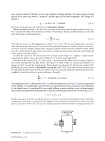
10.1.1 Boltzmann Transformation
In 1894 the famous Ludwig Boltzmann [1] showed that the nonlinear par-
tial differential equation (10.1) can be transformed to a nonlinear but ordi-
nary differential equation if
˜
D is a function of C(x) alone. He introduced the
variable
η ≡
x −x
M
2
√
t
, (10.2)
which is a combination of the space and time variables x and t, respectively.
x
M
refers to a special reference plane – the so-called Matano plane –tobe
defined below. Applying chain-rule differentiation to Eq. (10.1), we get the

following identity:
∂
∂x
≡
d
dη
∂η
∂x
=
1
2
√
t
d
dη
. (10.3)
The operator on the left-hand side of Eq. (10.1) is
∂
∂t
≡
d
dη
∂η
∂t
= −
x − x
M
4t
3/2
d

dη
= −
η
2t
d
dη
. (10.4)
The right-hand side of Eq. (10.1) can also be written in terms of η as
∂
∂x

˜
D(C)
∂C
∂x

=
d
dη
∂η
∂x

˜
D(C)
2
√
t
dC
dη


=
1
4t
d
dη

˜
D(C)
dC
dη

. (10.5)
10.1 Interdiffusion 163
Fig. 10.1. Schematic illustration of the Boltzmann-Matano method for a binary
diffusion couple with starting compositions C
L
and C
R
By recombining left- and right-hand sides and using the Boltzmann variable
we get Fick’s second law as an ordinary differential equation for C(η):
−2η
dC
dη
=
d
dη

˜
D(C)
dC

dη

. (10.6)
Some authors omit the factor 2 in the definition Eq. (10.2) of η. Then, a factor
of 1/2 instead of 2 appears in the equation corresponding to Eq. (10.6).
However, when finally transformed in ordinary time and space coordinates,
the solutions obtained are identical.
10.1.2 Boltzmann-Matano Method
The Boltzmann-transformed version of Fick’s second law Eq. (10.6) is a non-
linear ordinary differential equation. This equation allows us to deduce
the concentration-dependent interdiffusion coefficient from an experimen-
tal concentration-depth profile, C(x). Appropriate boundary conditions for
an interdiffusion experiment have been suggested by the Japanese scientist
Matano in 1933 [2]. He considered a binary diffusion couple, which consists
of two semi-infinite bars joined at time t = 0. The initial conditions are
C = C
L
for (x<0,t=0),
C = C
R
for (x>0,t=0). (10.7)
During a diffusion anneal of time t, a concentration profile C(x) develops.
This profile can be measured on a cross section of the diffusion zone, e.g., by
electron microprobe analysis (see Chap. 13). Such a profile is schematically
illustrated in Fig. 10.1.
164 10 Interdiffusion and Kirkendall Effect
Carrying out an integration between C
L
and a fixed concentration C
∗

,we
get from Eq. (10.6)
−2

C
∗
C
L
ηdC =
˜
D

dC
dη

C
∗
−
˜
D

dC
dη

C
L
. (10.8)
Matano’s geometry guarantees vanishing gradients dC/dη as C
∗
approaches

C
L
(or C
R
). Using (dC/dη)
C
L
= 0 and solving Eq. (10.8) for
˜
D yields
˜
D(C
∗
)=−2

C
∗
C
L
ηdC
(dC/dη)
C=C
∗
. (10.9)
We transform Eq. (10.9) back to space and time coordinates using the Boltz-
mann variable Eq. (10.2) and get
˜
D(C
∗
)=−

1
2t

C
∗
C
L
(x −x
M
)dC
(dC/dx)
C
∗
. (10.10)
This relation is called the Boltzmann-Matano equation. It permits us to deter-
mine
˜
D for any C
∗
from an experimental concentration-distance profile. For
the analysis, the position of the Matano plane, x
M
, must be known. Carrying
out the integration between the limits C
L
and C
R
, we get from Eq. (10.6)

C

R
C
L
ηdC =0. (10.11)
Equation (10.11) can be considered as the definition of the Matano plane.
x
M
must be chosen in such a way that Eq. (10.11) is fulfilled.
In order to determine the Matano plane, we have to remember that at
the beginning of the experiment the concentration of the diffusing species
was C
L
(C
R
) on the left-hand (right-hand) side. Let us suppose, for example,
C
L
<C
R
. Then, at the end of the experiment, the surplus of the diffusing
species found on the left-hand side must have arrived by diffusion from the
right-hand side. The location of the Matano plane can be determined from
the conservation condition
x
M

−∞
[C(x) −C
L
]dx


 
gain
=
∞

x
M
[C
R
− C(x)] dx

 
loss
. (10.12)
When integrated by parts, the integrals in Eq. (10.12) transform to integrals
with C as the running variable instead of x. If we apply the Matano boundary
conditions Eq. (10.7), we get
(C
L
− C
R
)x
M
+
C
M

C
L

xdC +
C
R

C
M
xdC =0 , (10.13)
10.1 Interdiffusion 165
where C
M
denotes the concentration at the Matano plane. If we choose the
Matano plane as origin of the x-axis (x
M
= 0), the first term in Eq. (10.13)
vanishes. Then, the following integrals balance across the Matano plane:
C
M

C
R
xdC +
C
L

C
M
xdC =0. (10.14)
Although the location of the Matano plane is not known a priori, it can
be found from experimental concentration-distance data by balancing the
horizontally hatched areas in Fig. 10.1.

In summary, the determination of interdiffusion coefficients from an ex-
perimental concentration-distance profile via the Boltzmann-Matano method
requires the following steps:
1. Determine the position of the Matano plane from Eq. (10.11) and use
this position as the origin of the x-axis.
2. Choose C
∗
and determine the integral

C
∗
C
L
xdC from the experimen-
tal concentration-distance data. The integral corresponds to the double-
hatched area A
∗
in Fig. 10.1.
3. Determine the concentration gradient S =(dC/dx)
C
∗
. S corresponds to
the slope of the concentration-distance curve at the position x
∗
.
4. Determine the interdiffusion coefficient
˜
D for C = C
∗
from the Boltz-

mann-Metano equation (10.10) as:
˜
D(C
∗
)=−A
∗
/(2tS).
We draw the readers attention to the following points:
(i) The Boltzmann-Matano equation (10.10) refers to an ‘infinite’ system.
Its application to an experiment requires that the concentration changes
must not have reached the boundaries of the system.
(ii) Close to the end-member compositions, the Boltzmann-Matano proce-
dure may incur relatively large errors in
˜
D because far away from the
Matano plane both the integral A
∗
and the slope S become very small.
(iii) The initial interface of a diffusion couple can be tagged by inert diffu-
sion markers (e.g., ThO
2
particles, thin Mo or W wires). The plane of
the markers in the diffusion couple is denoted as the Kirkendall plane.
Usually, for t = 0 the positions of the Matano plane and of the Kirk-
endall plane will be different. This is called the Kirkendall effect and is
discussed in Sect. 10.2.
(iv) This method is applicable when the volume of the diffusion couple does
not change during interdiffusion.
The Boltzmann-Matano method has been modified by Sauer and Freise [3]
and later by den Broeder [4]. These authors introduce a normalised con-

centration variable Y defined by:
Y =
C − C
R
C
L
− C
R
. (10.15)