Diffusion Solids Fundamentals Diffusion Controlled Solid State Episode 1 Part 10 pdf
Bạn đang xem bản rút gọn của tài liệu. Xem và tải ngay bản đầy đủ của tài liệu tại đây (766.58 KB, 25 trang )
218 13 Direct Diffusion Studies
The best way to determine the resulting concentration-depth profile is
serial sectioning of the sample and subsequent determination of the amount
of tracer per section. To understand sectioning the reader should think in
terms of isoconcentration contours. For lattice diffusion these are parallel to
the original surface, on which the thin layer is deposited, and perpendicu-
lar to the diffusion direction. The most important criterion of sectioning is
the parallelness of sections to the isococentration contours. For radioactive
tracers the specific activity per section, A(x), is proportional to the tracer
concentration:
A(x)=kC(x) . (13.8)
Here k is a constant, which depends on the nature and energy of the nuclear
radiation and on the efficiency of the counting device. The specific activ-
ity is obtained from the section mass and the count rate. The latter can
be measured in nuclear counting facilities such as γ-orβ-counting devices.
Usually, the count-rate must be corrected for the background count-rate of
the counting device. For short-lived radioisotopes half-life corrections are also
necessary. According to Eq. (13.4) a diagram of the logarithm of the specific
activity versus the penetration distance squared is linear. From its slope,
(4Dt)
−1
, and the diffusion time the tracer diffusivity D is obtained.
In an ordinary thin-layer sectioning experiment, one wishes to measure
diffusion over a drop of about three orders of magnitude in concentration.
About twenty sections suffice to define a penetration profile. The section
thickness ∆x required to get a concentration decrease of three orders of mag-
nitude over 20 sections is ∆x ≈
√
Dt/3.8. Thicker sections should be avoided
for the following reason: in a diffusion penetration profile the average con-
centrations (specific activities) per section are plotted versus the position of
the distance of the center of each section from the surface. Errors caused by
this procedure are only negligible if the sections are thin enough.
The radiotracer deposited on the front face of a sample may rapidly reach
the side surfaces of a sample by surface diffusion or via transport in the
vapour phase and then diffuse inward. To eliminate lateral diffusion effects,
one usually removes about 6
√
Dt from the sample sides before sectioning. For
studies of bulk diffusion, single crystalline samples rather than polycrystalline
ones should be used to eliminate the effects of grain-boundary diffusion, which
is discussed in Chap. 31. If no single crystals are available coarse-grained
polycrystals should be used.
The following serial-sectioning techniques are frequently used for the de-
termination of diffusion profiles:
Mechanical sectioning: For diffusion lengths,
√
Dt, of at least several mi-
crometers mechanical techniques are applicable (for a review see [4]). Lathes
and microtomes are appropriate for ductile samples such as some pure met-
als (Na, Al, Cu, Ag, Au, ) or polymers. For brittle materials such as
intermetallics, semiconductors, ionic crystals, ceramics, and inorganic glasses
grinding is a suitable technique.
13.3 Tracer Diffusion Experiments 219
Fig. 13.4. Penetration profile of the radioisotope
59
Fe in Fe
3
Si obtained by grinder
sectioning [15]. The solid line represents a fit of the thin-film solution of Fick’s
second law
For extended diffusion anneals and large enough diffusivities, D>
10
−15
m
2
s
−1
, lathe sectioning can be used. Diffusivities D>10
−17
m
2
s
−1
are accessible via microtome sectioning. In cases where the half-life of the
isotope permits diffusion anneals of several weeks, grinder sectioning can be
used for diffusivities down to 10
−18
m
2
s
−1
. Figure 13.4 shows a penetration
profile of the radioisotope
59
Fe in the intermetallic Fe
3
Si, obtained by grinder
sectioning [15]. Gaussian behaviour as stated by Eq. (13.4) is observed over
several orders of magnitude in concentration.
Ion-beam Sputter Sectioning (IBS): Diffusion studies at lower tempera-
tures often require measurements of very small diffusivities. Measurements of
diffusion profiles with diffusion lengths in the micrometer or sub-micrometer
range are possible using sputtering techniques. Devices for serial sectioning
of radioactive diffusion samples by ion-beam sputtering (IBS) are described
in [16, 17]. Figure 13.6 shows a schematic drawing of such a device. Oblique
incidence of the ion beam and low ion energies between 500 and 1000 eV are
used to minimise knock-on and surface roughening effects. The sample (typ-
ically several mm in diameter) is rotated to achieve a homogeneous lateral
sputtering rate. The sputter process is discussed in some detail below and
220 13 Direct Diffusion Studies
Fig. 13.5. Penetration profile of the radioisotope
59
Fe in Fe
3
Al obtained by sputter
sectioning [18]. The solid line represents a fit of the thin-film solution of Fick’s
second law
illustrated in Fig. 13.8, in connection with secondary ion mass spectroscopy
(SIMS). An advantage of IBS devices lies in the fact that neutral atoms are
collected, which comprise by far the largest amount (about 95 to 99 %) of
the off-sputtered particles. In contrast, SIMS devices (see below) analyse the
small percentage of secondary ions, which depends strongly on sputter- and
surface conditions.
Sectioning of shallow diffusion zones, which correspond to average diffu-
sion lengths between several ten nm and 10 µm, is possible using IBS devices.
For a reasonable range of annealing times up to about 10
6
s, a diffusivity range
between 10
−23
m
2
s
−1
and 10
−16
m
2
s
−1
can be examined. Depth calibration
can be performed by measuring the weight loss during the sputtering process
or by determining the depth of the sputter crater by interference microscopy
or by profilometer techniques. The depth resolution of IBS and SIMS is lim-
ited by surface roughening and atomic mixing processes to about several nm.
A penetration profile of
59
Fe in the intermetallic Fe
3
Al [18], obtained with
the sputtering device described in [17] is displayed in Fig. 13.5.
From diffusion profiles of the quality of Figs. 13.4 and 13.5, diffusion
coefficients can be determined with an accuracy of a few percent. A determi-
13.3 Tracer Diffusion Experiments 221
Fig. 13.6. Ion-beam sputtering device for serial sectioning of diffusion samples
nation of the absolute tracer concentration is not necessary since the diffusion
coefficient is obtained from the slope, −1/(4Dt), of such profiles.
Deviations from Gaussian behaviour in experimental penetration profiles
(not observed in Figs. 13.4 and 13.5) may occur for several reasons:
1. Grain-boundary diffusion: Grain boundaries in a polycrystalline sample
act as diffusion short-circuits with enhanced mobility of atoms. Grain
boundaries usually cause a ‘grain-boundary tail’ in the deeper penetrat-
ing part of the profile (see Chap. 32 and [19]). In the ‘tail’ region the
concentration of the diffuser is enhanced with respect to lattice diffusion.
Then, one should analyse the diffusion penetration profile in terms of
lattice diffusion and short-circuit diffusion terms:
C(x, t)=
M
√
πDt
exp
−
x
2
4Dt
+ C
0
exp(−Ax
6/5
) . (13.9)
Here C
0
is constant, which depends on the density of grain bound-
aries. The quantity A is related to the grain-boundary diffusivity, the
grain-boundary width, and to the lattice diffusivity. The grain-boundary
tails can be used for a systematic study of grain-boundary diffusion in
bi- or polycrystalline samples. Grain-boundary diffusion is discussed in
Chap. 32.
2. Evaporation losses of tracer : A tracer with high vapour pressure will
simultaneously evaporate from the surface and diffuse into the sample.
Then, the thin-film solution (13.4) is no longer valid. The outward flux of
the tracer will be proportional to the tracer concentration at the surface:
D
∂C
∂x
x=0
= −KC(0) . (13.10)
222 13 Direct Diffusion Studies
K is the rate constant for evaporation. The solution for Fick’s second
equation for this boundary condition is [1]
C(x, t)=M
1
√
πDt
exp
−
x
2
4Dt
−
K
D
exp
K
2
D
2
Dt +
K
D
x
erfc
x
2
√
Dt
+
K
D
√
Dt
. (13.11)
Evaporation losses of the tracer cause negative deviations from Gaussian
behaviour in the near-surface region.
3. Evaporation losses of the matrix : For a matrix material with a high
vapour pressure the surface of the sample may recede due to evaporation.
A solution for continuous matrix removal at a rate v and simultaneous
in-diffusion of the tracer has been given by [20]
C(x
,t)=M
1
√
πDt
exp(−η
2
) −
v
2D
erfc(η)
, (13.12)
where x
isthedistancefromthesurfaceafterdiffusionandη =(x
+
vt)/2
√
Dt.
13.3.2 Residual Activity Method
Gruzin has suggested a radiotracer technique, which is called the residual ac-
tivity method [21]. Instead of analysing the activity in each removed section,
the activity remaining in the sample after removing a section is measured.
This method is applicable if the radiation being detected is absorbed expo-
nentially. The residual activity A(x
n
) after removing a length x
n
from the
sample is then given by
A(x
n
)=k
∞
x
n
C(x)exp[−µ(x −x
n
)]dx, (13.13)
where k is a constant and µ is the absorption coefficient. According to
Seibel [22] the general solution of Eq. (13.13) – independent of the func-
tional form of C(x) – is given by
C(x
n
)=kA(x
n
)
µ −
dlnA(x
n
)
dx
n
. (13.14)
If the two bracket terms in Eq. (13.14) are comparable, the absorption co-
efficient must be measured accurately in the same geometry in which the
sample is counted. Thus, the Gruzin method is less desirable than counting
the sections, except for two limiting cases:
1. Strongly absorbed radiation: Suppose that the radiation is so weak that it
is absorbed in one section, i.e. µ dlnA(x
n
)/dx
n
.Isotopessuchas
63
Ni,
13.4 Isotopically Controlled Heterostructures 223
14
C, or
3
Hemitweakβ-radiation. Their radiation is readily absorbed and
Eq. (13.14) reduces to
C(x
n
)=µkA(x
n
) (13.15)
and the residual activity A(x
n
) follows the same functional form as C(x
n
).
In this case, the Gruzin technique has the advantage that it obviates the
tedious preparation of sections for counting.
2. Slightly absorbed radiation:Forµ dlnA(x
n
)/dx
n
the radiation is so
energetic that absorption is negligible. Then, the activity A
n
in section
n is obtained by subtracting two subsequent residual activities:
A
n
= A(x
n
) −A(x
n+1
) . (13.16)
The Gruzin technique is useful, when the specimen can be moved to the
counter repeatedly without loosing alignment in the sectioning device. In
general, this method is not as reliable as sectioning and straightforward mea-
surement of the section activity.
13.4 Isotopically Controlled Heterostructures
The use of enriched stable isotopes combined with modern epitaxial growth
techniques enables the preparation of isotopically controlled heterostructures.
Either chemical vapour deposition (CVD) or molecular beam epitaxy (MBE)
are used to produce the desired heterostructures. After diffusion annealing,
the diffusion profiles can be studied using, for example, conventional SIMS
or TOF-SIMS techniques (see the next section).
We illustrate the benefits of this method with an example of Si self-
diffusion. In the past, self-diffusion experiments were carried out using the
radiotracer
31
Si with a half-life of 2.6 hours. However, this short-lived radio-
tracer limits such studies to a narrow high-temperature range near the melt-
ing temperature of Si. Other self-diffusion experiments utilising the stable
isotope
30
Si (natural abundance in Si is about 3.1 %) in conjunction with neu-
tron activation analysis, SIMS profiling and nuclear reaction analysis (NRA)
overcame this diffuculty (see also Chap. 23). However, these methods have
the disadvantage that the
30
Si background concentration is high.
Figure 13.7 illustrates the technique of isotopically controlled heterostruc-
tures for Si self-diffusion studies. The sample consists of a Si-isotope het-
erostructure, which was grown by chemical vapour deposition on a natural
floating-zone Si substrate. A 0.7 µmthick
28
Si layer was covered by a layer
of natural Si (92.2 %
28
Si, 4.7 %
29
Si, 3.1 %
30
Si). The
28
Si profile in the as-
grown state (dashed line), after a diffusion anneal (crosses), and the best fit
to the data (solid line) are shown. Diffusion studies on isotopically controlled
heterostructures have been used by Bracht and Haller and their asso-
ciates mainly for self- and dopant diffusion studies in elemental [24, 25] and
compound semiconductors [26–28].
224 13 Direct Diffusion Studies
Fig. 13.7. SIMS depth profiles of
30
Si measured before and after annealing at
925
◦
C for 10 days of a
28
Si isotope heterostructure. The initial structure consisted
of a layer of
28
Si embedded in natural Si
13.5 Secondary Ion Mass Spectrometry (SIMS)
Secondary ion mass spectroscopy (SIMS) is an analytical technique whereby
layers of atoms are sputtered off from the surface of a solid, mainly as neu-
tral atoms and a small fraction as ions. Only the latter can be analysed in
a mass spectrometer. Several aspects of the sputtering process are illustrated
in Fig. 13.8. The primary ions (typically energies of a few keV) decelerate
during impact with the target by partitioning their kinetic energy through
a series of collisions with target atoms. The penetration depth of the primary
ions depends on their energy, on the types of projectile and target atoms and
their atomic masses, and on the angle of incidence. Each primary ion initiates
a ‘collision cascade’ of displaced target atoms, where momentum vectors can
be in any direction. An atom is ejected after the sum of phonon and colli-
sional energies focused on a target atom exceeds some threshold energy. The
rest of the energy dissipates into atomic mixing and heating of the target.
The sputtering yield of atomic and molecular species from a surface de-
pends strongly on the target atoms, on the primary ions and their energy.
Typical yields vary between 0.1 to 10 atoms per primary ion. The great ma-
jority of emitted atoms are neutral. For noble gas primaries the percentage of
secondary ions is below 1 %. If one uses reactive primary ions (e.g., oxygen-
or alkali-ions) the percentage of secondary ions can be enhanced through
the interaction of a chemically reactive species with the sputtered species by
exchanging electrons.
In a SIMS instrument, schematically illustrated in Fig. 13.9, a primary
ion beam hits the sample. The emitted secondary ions are extracted from
the surface by imposing an electrical bias of a few kV between the sample
13.5 Secondary Ion Mass Spectrometry (SIMS) 225
Fig. 13.8. Sputtering process at a surface of a solid
and the extraction electrode. The secondary ions are then transferred to the
spectrometer via a series of electrostatic and magnetic lenses. The spectrom-
eter filters out all but those ions with the chosen mass/charge ratios, which
are then delivered to the detector for counting. The classical types of mass
spectrometers are equipped either with quadrupole filters, or electric and
magnetic sector fields.
Time-of-flight (TOF) spectrometers are used in TOF-SIMS instruments.
The TOF-SIMS technique developed mainly by Benninghoven [35] com-
bines high lateral resolution (< 60 nm) with high depth resolution (< 1nm).
It is nowadays acknowledged as one of the major techniques for the surface
characterisation of solids. In different operational modes - surface spectrom-
etry, surface imaging, depth profiling - this technique offers several features:
the mass resolution is high; in principle all elements and isotopes can be de-
tected and also chemical information can be obtained; detection limits in the
range of ppm of a monolayer can be achieved. For details of the construction
of SIMS devices we refer to [33, 34, 36, 37].
When SIMS is applied for diffusion profile measurements, the mass spec-
trum is scanned and the ion current for tracer and host atoms can be recorded
simultaneously. In conventional SIMS, the ion beam is swept over the sample
and, in effect, digs a crater. An aperture prevents ions from the crater edges
from reaching the mass spectrometer. The diffusion profile is constructed from
the plots of instantaneous tracer/host atom ratio versus sputtering time. The
distance is deduced from a measurement of the total crater depth, assuming
that the material is removed uniformly as a function of time. Large changes
of the chemical composition along the diffusion direction can invalidate this
assumption.
226 13 Direct Diffusion Studies
Fig. 13.9. SIMS technique (schematic illustration)
One must keep in mind that the relationship between measured secondary-
ion signals and the composition of the target is complex. It involves all as-
pects of the sputtering process. These include the atomic properties of the
sputtered ions such as ionisation potentials, electron affinities, the matrix
composition of the target, the environmental conditions during the sputter-
ing process such as the residual gas components in the vacuum chamber, and
instrumental factors. Diffusion analysis by SIMS also depends on the accu-
racy of measuring the depth of the eroded crater and the resolution of the
detected concentration profile. A discussion of problems related to quantifi-
cation and standardisation of composition and distance in SIMS experiments
can be found in [34, 39].
SIMS, like the IBS technique discussed above, enables the measurement
of very small diffusion coefficients, which are not attainable with mechanical
sectioning techniques. The very good depth resolution and the high sensitivity
of mass spectrometry allows the resolution of penetration profiles of solutes
in the 10 nm range and at ppm level. Several perturbing effects, inherent to
the method and limiting its sensitivity are: degradation of depth resolution
by surface roughening, atomic mixing, and near surface distortion of profiles
by transient sputtering effects.
SIMS has mainly been applied for diffusion of foreign atoms although the
high mass resolution especially of TOF-SIMS also permits separation of stable
isotopes of the same element. SIMS has found particularly widespread use in
studies of implantation- and diffusion profiles in semiconductors. However,
SIMS is applicable to all kinds of solids. As an example, Fig. 13.10 shows
diffusion profiles for both stable isotopes
69
Ga and
71
Ga of natural Ga in
a ternary Al-Pd-Mn alloy (with a quasicrystalline structure) according to [38].
For metals, the relatively high impurity content of so-called ‘pure metals’ as
compared to semiconductors can limit the dynamic range of SIMS profiles.
13.6 Electron Microprobe Analysis (EMPA) 227
Fig. 13.10. Diffusion profiles for both stable isotopes
69
Ga and
71
Ga of natural
Ga in AlPdMn (icosahedral quasicrystalline alloy) according to [38]. The solid lines
represent fits of the thin-film solution
SIMS has in few cases also been applied to self-diffusion. This requires
that highly enriched stable isotopes are available as tracers. Contrary to self-
diffusion studies by radiotracer experiments, in the case of stable tracers
diffused into a matrix with a natural abundance of stable isotopes the latter
limits the concentration range of the diffusion profile. A fine example of this
technique can be found in a study of Ni self-diffusion in the intermetallic com-
pound Ni
3
Al, in which the highly enriched stable
64
Ni isotope was used [40].
The limitation due to the natural abundance of a stable isotope in the host
has been avoided in some SIMS studies of self-diffusion on amorphous Ni-
containing alloys by using the radioisotope
63
Ni as tracer [42, 43].
An elegant possibility to overcome the limits posed by the natural abun-
dance of stable isotopes are isotopically controlled heterostructures. This
method is discussed in the previous section and illustrated in Fig. 13.7.
13.6 Electron Microprobe Analysis (EMPA)
The basic concepts of electron microprobe analysis (EMPA) can be found
already in the PhD thesis of Castaing [44]. The major components of an
228 13 Direct Diffusion Studies
Fig. 13.11. Schematic view of an electron microprobe analyser (EMPA)
EMPA equipment are illustrated in Fig. 13.11. An electron-optical column
containing an electron gun, magnetic lenses, a specimen chamber, and vari-
ous detectors is maintained under high vacuum. The electron-optical column
produces a finely focused electron beam, with energies ranging between 10
and 50 keV. Scanning coils and/or a mechanical scanning device for the spec-
imen permit microanalysis at various sample positions. When the beam hits
the specimen it stimulates X-rays of the elements present in the sample. The
X-rays are detected and characterised either by means of an energy dispersive
X-ray spectrometer (EDX) or a crystal diffraction spectrometer. The latter
is also referred to as a wave-length dispersive spectrometer (WDX).
The ability to perform a chemical analysis is the result of a simple and
unique relationship between the wavelength of the characteristic X-rays, λ,
emitted from an element and its atomic number Z. It was first observed by
Moseley [45] in 1913. He showed that for K radiation
Z ∝
1
√
λ
. (13.17)
The origin of the characteristic X-ray emission is illustrated schematically in
Fig. 13.12. An incident electron with sufficient energy ejects a core electron
from its parent atom leaving behind an orbital vacancy. The atom is then
in an excited state. Orbital vacancies are quickly filled by electronic relax-
ations accompanied by the release of a discrete energy corresponding to the
difference between two orbital energy levels. This energy can be emitted as
an X-ray photon or it can be transferred to another orbital electron, called
13.6 Electron Microprobe Analysis (EMPA) 229
Fig. 13.12. Characteristic X-ray and Auger-electron production
an Auger electron, which is ejected from the atom. The fraction of electronic
relaxations which result in X-ray emission rather than Auger emission de-
pends strongly on the atomic number. It is low for small atomic numbers and
high for large atomic numbers. The characteristic radiation is superimposed
to the continuous radiation also denoted as ‘Bremsstrahlung’. The continuum
is the major source of the background and the principal factor limiting the
X-ray sensitivity. For details about EMPA, the reader may consult, e.g., the
reviews of Hunger [46] and Lifshin [47].
A diffusion profile is obtained by examining on a polished cross-section
of a diffusion sample the intensity of the characteristic radiation of the ele-
ment(s) involved in the diffusion process along the diffusion direction. The
detection limit in terms of atomic fractions is about 10
−3
to 10
−4
, depend-
ing on the selected element. It decreases with decreasing atomic number.
Light elements such as C or N are difficult to study because their fluores-
cence yield is low. The diameter of the electron beam is typically 1 µmor
larger depending on the instrument’s operating conditions. Accordingly, the
volume of X-ray generation is of the order of several µm
3
. This limits the
spatial resolution to above 1 to 2 µm. Thus, only relatively large diffusion
coefficients D>10
−15
m
2
s
−1
can be measured (Fig. 13.1). Because of its de-
tection limit, EMPA is mainly appropriate for interdiffusion- and multiphase-
diffusion studies. An example of a single-phase interdiffusion profile for an
Al
50
Fe
50
–Al
30
Fe
70
couple is shown in Fig. 13.13 [23].
The Boltzmann-Matano method [29, 30] is usually employed to evaluate
interdiffusion coefficients
˜
D from an experimental profile. Related procedures
for non-constant volume have been developed by Sauer and Freise and
den Broeder [31, 32]. These methods for deducing the interdiffusion coeffi-
cient,
˜
D(c), from experimental concentration-depth profiles are described in
Chap. 10.
230 13 Direct Diffusion Studies
Fig. 13.13. Interdiffusion profile of a Fe
70
Al
30
–Fe
50
Al
50
couple measured by EMPA
according to Salamon et al. [23]. Dashed line: composition distribution before the
diffusion anneal
13.7 Auger-Electron Spectroscopy (AES)
Auger-electron spectroscopy (AES) is named after Pierre Auger,whodis-
covered and explained the Auger effect in experiments with cloud chambers in
the mid 1920s (see [48]). An Auger electron is generated by transitions within
the electron orbitals of an atom following an excitation an electron from one
of the inner levels (see Fig. 13.12). Auger-electron spectroscopy (AES) was
introduced in the 1960s. In AES instruments the excitation is performed by
a primary electron beam.
The kinetic energy of the Auger electron is independent of the primary
beam but is characteristic of the atom and electronic shells involved in its
production. The probability that an Auger electron escapes from the surface
region decreases with decreasing kinetic energy. The range of analytical depth
in AES is typically between 1 and 5 nm. AES is one of the major techniques
for surface analysis.
When a primary electron beam strikes a surface, Auger electrons are only
a fraction of the total electron yield. Most of the electrons emitted from the
surface are either secondary electrons or backward scattered electrons. These
and the inelastically scattered Auger electrons constitute the background in
an Auger spectrum. Auger-electron emission and X-ray fluorescence after
creation of a core hole are competing processes and the emission probability
depends on the atomic number. The probability for Auger-electron emission
13.8 Ion-beam Analysis: RBS and NRA 231
Fig. 13.14. Schematic representation of Rutherford backscattering (RBS) and of
nuclear reaction analysis (NRA)
decreases with increasing atomic number whereas the probability for X-ray
fluorescence increases with atomic number. AES is thus particularly well
suited for light elements.
The combined operation of an AES spectrometer for chemical surface ana-
lysis and an ion sputtering device can be used for depth profiling. Information
with regard to the quantification and to factors affecting their resolution can
be found, e.g., in [49, 50]. AES is applicable to diffusion of foreign atoms,
since AES only discriminates between different elements. It has, for example,
been used to measure Au and Ag diffusion in amorphous Cu-Zr [41] and Cu
and Al diffusion in amorphous Zr
61
Ni
39
-alloys [51].
13.8 Ion-beam Analysis: RBS and NRA
High-energy ion-beam analysis has several desirable features for depth pro-
filing of diffusion samples. The technique is largely non-destructive, it offers
good depth resolution, and measurements of both concentration and depth
can be achieved. The depth resolution is in the range from about 0.01 to 1 µm.
This is inferior to the depth resolution achieved in IBS or SIMS devices but
substantially better than the resolution of mechanical sectioning techniques.
Atomic species are identified in ion-beam analysis by detecting the prod-
ucts of nuclear interactions, which are created by the incident MeV ions. There
are several different techniques. The two more important ones are Rutherford
backscattering (RBS) and nuclear reaction analysis (NRA). These two are
depicted schematically in Fig. 13.14.
232 13 Direct Diffusion Studies
Rutherford Backscattering (RBS): The first scattering experiment was
performed by Rutherford in 1911 [53] and his students Geiger and
Marsden [54] for verifications of the atomic model. A radioactive source
of α-particles was used to provide energetic probing ions and the particles
scattered from a gold foil were observed with a zinc blende scintillation
screen. Nowadays, elastic backscattering analysis also denoted as Ruther-
ford backscattering (RBS) is probably the most frequently used ion-beam
analytical technique among the surface analysis tools.
In RBS experiments a high-energy beam of monoenergetic ions (usually
α-particles) with energies of some MeV is used for depth profiling. The sam-
ple is bombarded along the diffusion direction with ions and one studies the
number of elastically backscattered ions as a function of their energy. The
particles of the analysing beam are scattered by the nuclei in the sample and
the energy spectrum of scattered particles is used to determine the concen-
tration profile of scattering nuclei. The signals from different nuclei can be
separated in the energy spectrum, because of the different kinematic factors
K of the scattering process. K is related to the masses of analysing particles
and scattering nuclei. It is a monotonically decreasing function of the mass
of the target nuclei. The backscattered particles re-emerge unchanged except
for a reduction in energy. The depth information comes from the continuous
energy loss of the ions in the sample. The yield of the backscattered ions is
proportional to the concentration of the scattering nuclei.
RBS is illustrated schematically in Fig. 13.15 for a layer of heavy atoms
(mass M) deposited on a substrate of light atoms (Mass m). Yield and en-
ergy of the backscattered ions are monitored by an energy-sensitive particle
detector and a multichannel analyser. The high energy end of the spectrum
(M-signal) corresponds to ions backscattered from heavy atoms at the sample
surface. The low energy end of the M -signal corresponds to ions backscat-
tered from the heavy atoms near the interface. The signals from the heavy
and light nuclei are separated in the spectrum due to the different kinematic
factors for heavy and light nuclei.
Although widely applicable, RBS has two inherent limitations for diffusion
studies: First, the element of interest must differ in mass sufficiently – at
least several atomic masses – from other constituents of the sample. Second,
adequate sensitivity is achieved only when the solutes are heavier than the
majority constituents of the matrix. Then, the backscattering yield from the
diffuser appears at higher energies than the yield from the majority nuclei.
Therefore, RBS is particular suitable for detecting heavy elements in a matrix
of substantially lower atomic weight. Because of the limited penetration range
of ions (several micrometers) and the associated energy straggling in a solid,
only relatively small diffusion coefficients are accessible.
Nuclear Reaction Analysis (NRA): In a NRA profiling experiment mo-
noenergetic high-energy particles (protons, α-particles, . . . ) are used as in
RBS. NRA is applicable if the analysing particles undergo a suitable nu-
13.8 Ion-beam Analysis: RBS and NRA 233
Fig. 13.15. Rutherford backscattering spectrometry: high-energy ion beam, elec-
tronics for particle detection and a schematic example of a RBS spectrum. The
technique is illustrated for a thin layer of atoms with mass M deposited on a sub-
strate of lower mass m
clear reaction with narrow resonance with the atoms of interest. The yield
of out-going reaction products is measured as a function of the energy of the
incident beam. From the yield versus energy curve the concentration profile
can be deduced.
As shown schematically in Fig. 13.14, the analysis-beam particles un-
dergo an inelastic, exothermic nuclear reaction with the target nuclei thus
producing two or more new particles. Depending on the conditions it may
be preferable to detect either charged reaction products, neutrons or γ-rays
from the reaction. This method distinguishes specific isotopes and is there-
fore free from the mass-related restrictions of RBS. Suitable resonant nuclear
reactions occur for at least one readily available isotope of all elements from
hydrogen to fluorine and for beam energies below 2 MeV. NRA can mainly
be used to investigate the diffusion of light solutes in a heavier matrix.
Concluding Remarks: Depth profiling is possible in RBS and NRA be-
cause the charged particles continuously loose energy as they traverse the
specimen. Usually, this loss is almost entirely due to electronic excitations,
although there is some additional contribution from small-angle nuclear scat-
tering. The consequences may be appreciated by considering the RBS ex-
periment illustrated in Fig. 13.15. In RBS the energy of the analysis-beam
particle decreases during both inward and outward passages. When the par-
ticle is detected, the accumulated energy loss is superimposed on the recoil
234 13 Direct Diffusion Studies
loss via the kinematic factor. Hence the measured energy decreases mono-
tonically with the depth of the scattering nucleus. In NRA the situations are
analogous but more varied. For example, the relevant energy loss may occur
only during the inward or outward passage. Nevertheless, depth resolution is
always a consequence of the charged-particle energy loss in the sample. For
example, the diffusion of ion-implanted boron in amorphous Ni
59.5
Nb
40.5
was
measured by irradiating the amorphous alloy with high energy protons and
detecting α-particles emitted from the nuclear reaction
11
B+p→
8
B+α,
and determining the concentration profile of
11
B from the number and energy
of emitted α-particles as a function of the incident proton energy [52].
In NRA and in RBS the penetration range of ions is not more than several
micrometer. This limits the diffusion depth. Diffusion coefficients between
about 10
−17
and 10
−23
m
2
s
−1
are accessible (see also Fig. 13.1). Both RBS
and NRA methods need a depth calibration, which is based on not always very
accurate data of the stopping power in the matrix for the relevant particles.
Also the depth resolution is usually inferior to that achievable in careful IBS
radiotracer and SIMS profiling studies. For a comprehensive discussion of ion-
beam techniques the reader may consult reviews by Myers [55], Lanford
et al. [56], and Chu et al. [57].
References
1. J. Crank, The Mathematics of Diffusion, Oxford University Press, 2nd ed., 1975
2. J. Philibert, Atom Movements – Diffusion and Mass Transport in Solids,Les
Editions de Physique, Les Ulis, 1991
3. Th. Heumann, Diffusion in Metallen, Springer-Verlag, Berlin, 1992
4. S.J. Rothman, The Measurement of Tracer Diffusion Coefficients in Solids,
in: Diffusion in Crystalline Solids, G.E. Murch, A.S. Nowick (Eds.), Academic
Press, 1984, p. 1
5. H. Mehrer (Vol. Ed.), Sect. 1.6 in: Diffusion in Solid Metals and Alloys,
Landolt-B¨ornstein, Numerical Data and Functional Relationships in Science
and Technology, New Series, Group III: Crystal and Solid State Physics, Vol.
26, Springer-Verlag, 1990
6. Proc. Int. Conf. on Diffusion in Materials – DIMAT-92, Kyoto, Japan, 1992,
M. Koiwa, H. Nakajima, K I. Hirano (Eds.); also: Defect and Diffusion Forum
95–98 (1993)
7. Proc. Int. Conf. on Diffusion in Materials – DIMAT-96, Nordkirchen, Germany,
1996, H. Mehrer, Chr. Herzig, N.A. Stolwijk, H. Bracht (Eds.); also: Defect and
Diffusion Forum 143–147 (1997)
8. Proc. Int. Conf. on Diffusion in Materials – DIMAT-2000, Paris, France, 2000,
Y. Limoge, J.L. Bocquet (Eds.); also: Defect and Diffusion Forum 194–199
(2001)
9. Proc. Int. Conf. on Diffusion in Materials – DIMAT-2004, Cracow, Poland,
2004, M. Danielewski, R. Filipek, R. Kozubski, W. Kucza, P. Zieba, Z. Zurek
(Eds.); also: Defect and Diffusion Forum 237–240 (2005)
10. H. Mehrer, Materials Transactions, JIM, 37, 1259 (1996)
References 235
11. H.Mehrer,F.Wenwer,Diffusion in Metals,in:Diffusion in Condensed Matter,
J. K¨arger, R. Haberlandt, P. Heitjans (Eds.), Vieweg Verlag, 1998
12. H. Mehrer, Diffusion: Introduction and Case Studies in Metals and Binary
Alloys,in:Diffusion in Condensed Matter – Methods, Materials, Models,P.
Heitjans, J. K¨arger (Eds.), Springer-Verlag, 2005
13. D. Tannhauser, J. Appl. Phys. 27, 662 (1956)
14. H. Mehrer, Phys. Stat. Sol. (a) 104, 247 (1987)
15. A. Gude, H. Mehrer, Philos. Mag. A 76, 1 (1996)
16. F. Faupel, P.W. H¨uppe, K. R¨atzke, R. Willecke. T. Hehenkamp, J. Vac. Sci.
Technol. a 10, 92 (1992)
17. F.Wenwer,A.Gude,G.Rummel,M.Eggersmann,Th.Zumkley,N.A.Stolwijk,
H. Mehrer, Meas. Sci. Technol. 7, 632 (1996)
18. M. Eggersmann, B. Sepiol, G. Vogl, H. Mehrer, Defect and Diffusion Forum
143–147, 339 (1997)
19. I. Kaur, Y. Mishin, W. Gust, Fundamentals of Grain and Interphase Boundary
Diffusion, John Wiley & Sons Ltd., 1995
20. R.N. Ghoshtagore, Phys. Stat. Sol. 19, 123 (1967)
21. P.L. Gruzin, Dokl. Akad. Nauk. SSSR 86, 289 (1952)
22. G. Seibel, Int. J. Appl. Radiat. Isot. 15, 679 (1964)
23. M. Salamon, S. Dorfman, D. Fuks, G. Inden, H. Mehrer, Defect and Diffusion
Forum 194–199, 553 (2001)
24. H.D. Fuchs, W. Walukiewicz, E.E. Haller, W. Dondl, R. Schorer, G. Abstreiter,
A.I. Rudnev, A.V. Tikomirov, V.I. Ozhogin, Phys. Rev. B51, 16817 (1995)
25. H. Bracht, E.E. Haller, R. Clark-Phelps, Phys. Rev. Lett. 81 393 (1998)
26. L. Wang, L. Hsu, E.E. Haller, J.W. Erickson, A. Fisher, K. Eberl, M. Cardona,
Phys. Rev. Lett. 76, 2342 (1996)
27. L.Wang,J.A.Wolk,L.Hsu,E.E.Haller,J.W.Erickson,M.Cardona,T.Ruf,
J.P. Silveira, F. Briones, Appl. Phys. Lett. 70, 1831 (1997)
28. H. Bracht, E.E. Haller, K. Eberl, M. Cardona, R. Clark-Phelps, Mat. Res. Soc.
Symp. 527, 335 (1998)
29. L. Boltzmann, Wiedemanns Ann. Physik 53, 959 (1894)
30. C. Matano, Jap. J. Phys. 8, 109–113 (1933)
31. F. Sauer, V. Freise, Z. Elektrochem. 66, 353 (1962)
32. F.J.A. den Broeder, Scr. Metall. 3, 321 (1969)
33. C E. Richter, Sekund¨arionen-Massenspektroskopie und Ionenstrahl-Mikroana-
lyse,in:Ausgew¨ahlte Untersuchungsverfahren der Metallkunde, H J. Hunger
et al. (Eds.), VEB Verlag, 1983, p. 197
34. W.T. Petuskey, Diffusion Analysis using Secondary Ion Mass Spectroscopy,in:
Nontraditional Methods in Diffusion, G.E. Murch, H.K. Birnbaum, J.R. Cost
(Eds.), The Metallurgical Society of AIME, Warrendale, 1984, p. 179
35. A. Benninghoven, The History of Static SIMS: a Personal Perspective,in:TOF-
SIMS – Surface Analysis by Mass Spectrometry, J.C. Vickerman, D. Briggs
(Eds.), IM Publications and Surface Spectra Limited, 2001
36. A. Benninghoven, F.G. R¨udenauer, H.W. Werner, Secondary Ion Mass Spec-
trometry – Basic Concepts, Instrumental Aspects, Applications and Trends,
John Wiley and Sons, Inc., 1987
37. J.C. Vickerman, D. Briggs (Eds.), TOF-SIMS – Surface Analysis by Mass Spec-
trometry, IM Publications and Surface Spectra Limited, 2001
236 13 Direct Diffusion Studies
38. H. Mehrer, R. Galler, W. Frank, R. Bl¨uher, T. Strohm, Diffusion in Quasicrys-
tals,in:Quasicrystals: Structure and Physical Properties, H R. Trebin (Ed.),
J. Wiley VCH, 2003
39. M P. Macht, V. Naundorf, J. Appl. Phys. 53, 7551 (1982)
40. S. Frank, U. S¨odervall, Chr. Herzig, Phys. Stat. Sol. (b) 191, 45 (1995)
41. E.C. Stelter, D. Lazarus, Phys. Rev. B 36, 9545 (1987)
42. A.K. Tyagi, M P. Macht, V. Naundorf, Scripta Metall. et Mater. 24, 2369
(1999)
43. A.K. Tyagi, M P. Macht, V. Naundorf, Acta Metall. et Mater. 39, 609 (1991)
44. R. Castaing, Ph.D. thesis, Univ. of Paris, 1951
45. H.G.J. Moseley, Philos. Mag. 26, 1024 (1913)
46. H J. Hunger, Elektronenstrahl-Mikroanalyse und Rasterelektronen-Mikrosko-
pie,in:Ausgew¨ahlte Untersuchungsverfahren der Metallkunde, H J. Hunger
et al. (Eds.), VEB Deutscher Verlag f¨ur Grundstoffindustrie, Leipzig, 1983,
p.175
47. E. Lifshin, Electron Microprobe Analysis,in:Materials Science and Technol-
ogy, R.W. Cahn, P. Haasen, E.J. Kramer (Eds.), Vol. 2B: Characterisation of
Materials, VCH, 1994, p. 351
48. P. Auger, Surf. Sci 1, 48 (1975)
49. S. Hofmann, Surf. Interface Anal. 9, 3 (1986)
50. A. Zalar, S. Hofmann, Surf. Interface Anal. 12, 83 (1988)
51. S.K. Sharma, P. Mukhopadhyay, Acta Metall. 38, 129 (1990)
52. M.M. Kijek, D.W. Palmer, B. Cantor, Acta Metall. 34, 1455 (1986)
53. E. Rutherford, Philos. Mag. 21, 669 (1911)
54. H. Geiger, E. Marsden, Philos. Mag. 25, 206 (1913)
55. S.M. Myers, Ion-beam Analysis and Ion Implantation in the Study of Diffusion,
in: Nontraditional Methods in Diffusion,G.E.Murch,H.K.Birnbaum,J.R.Cost
(Eds.), The Metallurgical Society of AIME, Warrendale, 1984, p. 137
56. W.A. Lanford, R. Benenson, C. Burman, L. Wielunski, Nuclear Reaction
Analysis for Diffusion Studies,in:Nontraditional Methods in Diffusion,G.E.
Murch, H.K. Birnbaum, J.R. Cost (Eds.), The Metallurgical Society of AIME,
Warrendale, 1984, p. 155
57. W.K. Chu, J. Liu, Z. Zhang, K.B. Ma, High Energy Ion Beam Analysis Tech-
niques,in:Materials Science and Technology, R.W. Cahn, P. Haasen, E.J.
Cramer (Eds.), Vol. 2B: Characterisation of Materials, VCH Weinheim, 1994,
p. 423
14 Mechanical Spectroscopy
14.1 General Remarks
The discoveries of thermally-activated anelastic relaxation processes in solids
by Snoek [1], Zener [2,3]andGorski [4] were made more than half a cen-
tury ago. Since then, anelastic measurements have become an established
tool for the study of atomic movements in solids. Relaxation methods and
the closely related internal friction (or damping) methods make use of the
fact that atomic motion in a solid can be induced by the application of con-
stant or oscillating mechanical stress. Nowadays, anelastic measurements are
also denoted by the title mechanical spectroscopy.
Under the influence of an applied stress or strain, an instantaneous elastic
effect (Hooke’s law) is observed, followed by strain or stress which varies with
time. The latter effect is called anelasticity or anelastic relaxation. Anelastic
behaviour is reversible. If stress (strain) is removed the sample will return –
after some time – to its initial shape. This distinguishes anelastic from plastic
behaviour.
Light interstitials, such as H, C, N, and O as well as substitutional so-
lutes and solute-defect complexes are accompanied by local straining of the
surrounding lattice. The presence of microstrains surrounding a diffusing
atom allows interaction between a macroscopic stress field arising from ex-
ternal forces applied to the material. This interaction generates a rich va-
riety of stress-assisted diffusion effects. Stress-mediated motion can cause
time-dependent anelastic (recoverable) strains that result in several types of
internal friction processes encountered in many materials.
Sometimes, anelastic relaxation involves the reorientation of point defects
which act as elastic dipoles as illustrated in Fig. 14.1. Reorientation relax-
ations are short-range processes, which in some cases involve only one or few
atomic jump(s). However, only in some special cases, exemplified by Snoek re-
laxation, the same jump produces both reorientation and diffusion. Only then,
a simple relationship exists between the relaxation time and the long-range
diffusion coefficient. Long-range diffusion controls the so-called Gorski relax-
ation illustrated in Fig. 14.2. Gorsky relaxation can be produced by bending
a sample containing defects, which act as dilatation centers. In practice, the
only experimentally known example of Gorski relaxation is due to hydrogen
diffusion metals. It can be observed because hydrogen diffusion is very fast.
238 14 Mechanical Spectroscopy
Fig. 14.1. Schematic illustration of anelastic relaxation caused by reorientation of
elastic dipoles (represented by grey ellipses)
Fig. 14.2. Schematic illustration of Gorski-effect
One should, however, keep in mind that mechanical relaxation and in-
ternal friction may arise from various sources. These can range from point-
defect reorientations, long-range diffusion, dislocation effects, grain-boundary
processes, and phase transformations to visco-elastic behaviour and plastic
deformation. Some point-defect relaxations are diffusion-related, some are
not. For point-defect relaxations of trapped and paired defects, the nature
and the activation enthalpy of the reorientation jump can be significantly
different from those associated with long-range diffusion. A review of the
substantial body of work that has been accumulated on the study of atomic
movement by anelastic methods is beyond the scope of this chapter.
Several textbooks, e.g., those of Zener [3] and Nowick and Berry [5]
and reviews by Berry and Pritchet [6, 7] are available for the interested
reader. A review about the potential of mechanical loss spectroscopy for in-
organic glasses and glass ceramics has been given by Roling [8]. A compre-
hensive treatment of magnetic relaxation effects can be found in a textbook
of Kronm
¨
uller [9].
In the present chapter, we first mention the basic concepts of mechanical
loss spectroscopy, i.e. of anelastic behaviour and internal friction. Then, we
describe some examples of diffusion-related anelasticity such as the Snoek
effect,theZener effect,theGorski effect, and give an example of a mechanical
loss spectrum of glasses.
14.2 Anelasticity and Internal Friction 239
14.2 Anelasticity and Internal Friction
From the viewpoint of mechanical stress-strain behaviour, we may regard an
ideal solid as one which obeys Hooke’s law and thus behaves in an ideally
elastic manner. Such a solid would always recover completely and instanta-
neously on removal of an applied stress. If set into vibration, the solid would
vibrate forever with undiminished amplitude if totally isolated from its sur-
roundings. The mechanical behaviour of real solids at low stress levels (below
the yield stress) is modified by the appearance of anelasticity, which develops
at a rate controlled by the atomic movements. It can often be traced back to
the presence of mobile atoms or point defects.
A quantitative description of the anelastic behaviour of materials can be
found by analysing a model having the name standard linear solid,whichwas
originally proposed by Voigt [10] and by Poynting and Thomson [11].
In this model, stress σ,strain, and their respective time derivatives, ˙σ and
˙, are related through a linear response equation:
σ + τ
˙σ = M
R
( + τ
σ
˙) . (14.1)
This anelastic equation of state is a generalisation of Hooke’s law of linear
elasticity. Equation (14.1) contains three material parameters: the strain re-
laxation time τ
,thestress relaxation time τ
σ
(sometimes also denoted as
the stress retardation time), and the relaxed elastic modulus M
R
. Figure 14.3
illustrates in its left part the strain response of a standard linear solid in-
duced by an instantaneous application and subsequent removal of a constant
stress. The continued relaxation of the strain after removal of the stress is also
termed the elastic aftereffect. The stress response induced by instantaneous
application and removal of strain is illustrated in the right part. Note that
τ
σ
and τ
are different. It is obvious from Eq. (14.1) that for vanishing time
derivatives Eq. (14.1) reduces to Hooke’s law. Under uniaxial stress M
R
is
termed the Young modulus, whereas under applied shear M
R
is termed the
shear modulus.
Periodic Stress and Strain: Let us now suppose that a uniaxial, periodic
stress-time function of frequency ω and amplitude σ
0
of the form
σ = σ
0
exp [iωt] (14.2)
is imposed on the material. The time-dependent strain response of an anelas-
tic solid then is
=
0
exp [i(ωt − δ)] , (14.3)
where δ is the phase shift between σ and . For a completely elastic material,
σ and are in phase and the phase shift is zero for all frequencies. The stress-
strain behaviour for an anelastic material under periodic stress is illustrated
in Fig. 14.4. For an anelastic material a hysteresis loop is obtained. The area
240 14 Mechanical Spectroscopy
Fig. 14.3. Schematic illustration of anelastic behaviour. The strain response for
an instantaneous stress-time function is shown in the left half. The stress response
for an instantaneous strain-time function corresponds to the right half
Fig. 14.4. Stress-strain relations for a periodically driven anelastic material at
three different frequencies
inside the hysteresis represents the dissipated energy per unit volume and
per cycle (see below).
It is convenient to introduce a complex elastic modulus
ˆ
M via
σ =
ˆ
M, (14.4)
which can be split up according to
ˆ
M = M
+ iM
, (14.5)
i.e. into real and imaginary parts M
and M
, respectively. Assuming peri-
odic strain with a frequency ω and substituting Eqs. (14.4) and (14.5) into
Eq. (14.1) yields after a few steps of algebra
ˆ
M = M
R
1+τ
σ
iω
1+τ
iω
. (14.6)
14.2 Anelasticity and Internal Friction 241
After separation into real and imaginary parts we get
M
(ω)=M
R
1+τ
τ
σ
ω
2
1+ω
2
τ
2
= M
R
+∆M
ω
2
τ
2
1+ω
2
τ
2
(14.7)
and
M
(ω)=M
R
(τ
σ
− τ
)ω
1+ω
2
τ
2
=∆M
ωτ
1+ω
2
τ
2
, (14.8)
where the abbreviations
∆M ≡ M
U
− M
R
and ∆ ≡ ∆M/M
R
(14.9)
have been introduced. At high frequencies, the time scale for stress and
strain removals becomes small compared to the relaxation times. Then M
approaches an unrelaxed elastic modulus
M
U
=
M
R
τ
σ
τ
, (14.10)
which denotes the stress increment per unit strain at high frequency. Note
that M
U
and M
R
are different because τ
σ
and τ
are different. The tangent
of the loss angle δ is given by
tan δ ≡ M
/M
=∆M
ωτ
M
R
+ M
U
ω
2
τ
2
≡ ∆
ω(τ
σ
− τ
)
1+τ
σ
τ
ω
2
. (14.11)
Internal Friction: Internal friction is the dissipation of mechanical energy
caused by anelastic processes occurring in a strained solid. The internal fric-
tion, usually called Q
−1
, in a cyclically driven anelastic solid is defined as
Q
−1
≡
∆E
dissipated
E
stored
, (14.12)
where ∆E
dissipated
is the energy dissipated as heat per unit volume of the
material over one cycle. E
stored
denotes the peak elastic energy stored per
unit volume. For a periodically strained solid subject to sinusoidal stress, the
internal friction is given by the following ratio of energy integrals:
Q
−1
=
2π
0
σ(ωt)˙(ωt)
out−of−phase
d(ωt)
2π
0
σ(ωt)˙(ωt)
in−phase
d(ωt)
. (14.13)
Substituting the out-of-phase and in-phase components of the strain rate ˙
yields after some algebra the following relation between internal friction and
the tangent of the loss angle:
Q
−1
= π tan δ. (14.14)
242 14 Mechanical Spectroscopy
It is convenient to combine the stress and strain relaxation times to a mean
relaxation time τ, which is defined as the geometric mean of the two funda-
mental times:
τ ≡
√
τ
σ
τ
. (14.15)
We will see later that τ sometimes can be associated with atomic jump pro-
cesses occurring in the strained solid, having a well-defined activation en-
thalpy. It is also convenient to combine the relaxed and the unrelaxed moduli
to a mean modulus M via
M ≡
M
R
M
U
=
τ
σ
τ
M
R
=
τ
τ
σ
M
U
. (14.16)
Using the definitions of the mean modulus Eq. (14.16), the mean relaxation
time Eq. (14.15) and Eq. (14.11), yields a basic expression for internal friction:
Q
−1
= π tan δ = π
∆M
M
ωτ
1+ω
2
τ
2
. (14.17)
The term π∆M/M is called the relaxation strength. The second term de-
scribes the frequency dependence of internal friction. Figure 14.5 shows a di-
agram of Q
−1
versus the logarithm of ωτ. The frequency-dependent modulus
M
is also shown, which varies between the relaxed modulus M
R
at low fre-
quencies and the unrelaxed modulus M
U
at high frequencies. The maximum
of internal friction occurs when
ωτ = 1 (14.18)
is fulfilled. This relation is an important condition for the analysis of anelas-
ticity. If an anelastic solid is strained periodically with a frequency ω the
maximum energy loss occurs, when the imposed frequency and relaxation
time of the process match.
14.3 Techniques of Mechanical Spectroscopy
Usually, the relaxation time τ is thermally activated according to
τ ∝ exp
∆H
k
B
T
, (14.19)
where ∆H denotes some activation enthalpy. Thus, by varying the temper-
ature at constant frequency ω a maximum of internal friction occurs on the
temperature scale. This is the usual way of measuring internal friction peaks,
as temperature is easier to vary than frequency. The latter is often more or
less fixed by the internal friction device.
By using different experimental techniques, the mechanical loss can be
determined at frequencies roughly between 10
−5
and 5×10
10
Hz. It is conve-
nient to perform temperature-dependent measurements at fixed frequencies.