Foundations of Technical Analysis phần 3 potx

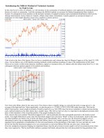
(a) Double Top
(b) Double Bottom
Figure 7. Double tops and bottoms.
Foundations of Technical Analysis 1725
III. Is Technical Analysis Informative?
Although there have been many tests of technical analysis over the years,
most of these tests have focused on the profitability of technical trading
rules.
9
Although some of these studies do find that technical indicators can
generate statistically significant trading profits, but they beg the question
of whether or not such profits are merely the equilibrium rents that accrue
to investors willing to bear the risks associated with such strategies. With-
out specifying a fully articulated dynamic general equilibrium asset-pricing
model, it is impossible to determine the economic source of trading profits.
Instead, we propose a more fundamental test in this section, one that
attempts to gauge the information content in the technical patterns of Sec-
tion II.A by comparing the unconditional empirical distribution of returns
with the corresponding conditional empirical distribution, conditioned on the
occurrence of a technical pattern. If technical patterns are informative, con-
ditioning on them should alter the empirical distribution of returns; if the
information contained in such patterns has already been incorporated into
returns, the conditional and unconditional distribution of returns should be
close. Although this is a weaker test of the effectiveness of technical analy-
sis—informativeness does not guarantee a profitable trading strategy—it is,
nevertheless, a natural first step in a quantitative assessment of technical
analysis.
To measure the distance between the two distributions, we propose two
goodness-of-fit measures in Section III.A. We apply these diagnostics to the
daily returns of individual stocks from 1962 to 1996 using a procedure de-
scribed in Sections III.B to III.D, and the results are reported in Sec-

tions III.E and III.F.
A. Goodness-of-Fit Tests
A simple diagnostic to test the informativeness of the 10 technical pat-
terns is to compare the quantiles of the conditional returns with their un-
conditional counterparts. If conditioning on these technical patterns provides
no incremental information, the quantiles of the conditional returns should
be similar to those of unconditional returns. In particular, we compute the
9
For example, Chang and Osler ~1994! and Osler and Chang ~1995! propose an algorithm for
automatically detecting head-and-shoulders patterns in foreign exchange data by looking at
properly defined local extrema. To assess the efficacy of a head-and-shoulders trading rule, they
take a stand on a class of trading strategies and compute the profitability of these across a
sample of exchange rates against the U.S. dollar. The null return distribution is computed by a
bootstrap that samples returns randomly from the original data so as to induce temporal in-
dependence in the bootstrapped time series. By comparing the actual returns from trading
strategies to the bootstrapped distribution, the authors find that for two of the six currencies
in their sample ~the yen and the Deutsche mark!, trading strategies based on a head-and-
shoulders pattern can lead to statistically significant profits. See, also, Neftci and Policano
~1984!, Pruitt and White ~1988!, and Brock et al. ~1992!.
1726 The Journal of Finance
deciles of unconditional returns and tabulate the relative frequency Zd
j
of
conditional returns falling into decile j of the unconditional returns, j ϭ
1, ,10:
Zd
j
[
number of conditional returns in decile j
total number of conditional returns

. ~15!
Under the null hypothesis that the returns are independently and identi-
cally distributed ~IID! and the conditional and unconditional distributions
are identical, the asymptotic distributions of Zd
j
and the corresponding goodness-
of-fit test statistic Q are given by
!
n~ Zd
j
Ϫ 0.10!;
a
N
~
0,0.10~1 Ϫ 0.10!
!
, ~16!
Q [
(
jϭ1
10
~n
j
Ϫ 0.10n!
2
0.10n
;
a
x
9

2
, ~17!
where n
j
is the number of observations that fall in decile j and n is the total
number of observations ~see, e.g., DeGroot ~1986!!.
Another comparison of the conditional and unconditional distributions of
returns is provided by the Kolmogorov–Smirnov test. Denote by $Z
1t
%
tϭ1
n
1
and
$Z
2t
%
tϭ1
n
2
two samples that are each IID with cumulative distribution func-
tions F
1
~z! and F
2
~z!, respectively. The Kolmogorov–Smirnov statistic is de-
signed to test the null hypothesis that F
1
ϭ F
2

and is based on the empirical
cumulative distribution functions
Z
F
i
of both samples:
Z
F
i
~z![
1
n
i
(
kϭ1
n
i
1~Z
ik
Յ z!, i ϭ 1,2, ~18!
where 1~{! is the indicator function. The statistic is given by the expression
g
n
1
, n
2
ϭ
ͩ
n
1

n
2
n
1
ϩ n
2
ͪ
10 2
sup
Ϫ`ϽzϽ`
6
Z
F
1
~z! Ϫ
Z
F
2
~z!6. ~19!
Under the null hypothesis F
1
ϭ F
2
, the statistic g
n
1
, n
2
should be small. More-
over, Smirnov ~1939a, 1939b! derives the limiting distribution of the statistic

to be
lim
min~n
1
, n
2
!r`
Prob~g
n
1
,n
2
Յ x! ϭ
(
kϭϪ`
`
~Ϫ1!
k
exp~Ϫ2k
2
x
2
!, x Ͼ 0. ~20!
Foundations of Technical Analysis 1727
An approximate a-level test of the null hypothesis can be performed by com-
puting the statistic and rejecting the null if it exceeds the upper 100ath
percentile for the null distribution given by equation ~20!~see Hollander and
Wolfe ~1973, Table A.23!, Csáki ~1984!, and Press et al. ~1986, Chap. 13.5!!.
Note that the sampling distributions of both the goodness-of-fit and
Kolmogorov–Smirnov statistics are derived under the assumption that re-

turns are IID, which is not plausible for financial data. We attempt to ad-
dress this problem by normalizing the returns of each security, that is, by
subtracting its mean and dividing by its standard deviation ~see Sec. III.C!,
but this does not eliminate the dependence or heterogeneity. We hope to
extend our analysis to the more general non-IID case in future research.
B. The Data and Sampling Procedure
We apply the goodness-of-fit and Kolmogorov–Smirnov tests to the daily
returns of individual NYSE0AMEX and Nasdaq stocks from 1962 to 1996
using data from the Center for Research in Securities Prices ~CRSP!.To
ameliorate the effects of nonstationarities induced by changing market struc-
ture and institutions, we split the data into NYSE0AMEX stocks and Nas-
daq stocks and into seven five-year periods: 1962 to 1966, 1967 to 1971,
and so on. To obtain a broad cross section of securities, in each five-year
subperiod, we randomly select 10 stocks from each of five market-
capitalization quintiles ~using mean market capitalization over the subperi-
od!, with the further restriction that at least 75 percent of the price
observations must be nonmissing during the subperiod.
10
This procedure
yields a sample of 50 stocks for each subperiod across seven subperiods
~note that we sample with replacement; hence there may be names in
common across subperiods!.
As a check on the robustness of our inferences, we perform this sampling
procedure twice to construct two samples, and we apply our empirical analy-
sis to both. Although we report results only from the first sample to con-
serve space, the results of the second sample are qualitatively consistent
with the first and are available upon request.
C. Computing Conditional Returns
For each stock in each subperiod, we apply the procedure outlined in Sec-
tion II to identify all occurrences of the 10 patterns defined in Section II.A.

For each pattern detected, we compute the one-day continuously com-
pounded return d days after the pattern has completed. Specifically, con-
sider a window of prices $P
t
% from t to t ϩ l ϩ d Ϫ 1 and suppose that the
10
If the first price observation of a stock is missing, we set it equal to the first nonmissing
price in the series. If the tth price observation is missing, we set it equal to the first nonmissing
price prior to t.
1728 The Journal of Finance
identified pattern p is completed at t ϩ l Ϫ 1. Then we take the conditional
return R
p
as log~1 ϩ R
tϩlϩdϩ1
!. Therefore, for each stock, we have 10 sets of
such conditional returns, each conditioned on one of the 10 patterns of
Section II.A.
For each stock, we construct a sample of unconditional continuously com-
pounded returns using nonoverlapping intervals of length t, and we compare
the empirical distribution functions of these returns with those of the con-
ditional returns. To facilitate such comparisons, we standardize all returns—
both conditional and unconditional—by subtracting means and dividing by
standard deviations, hence:
X
it
ϭ
R
it
Ϫ Mean@R

it
#
SD@R
it
#
, ~21!
where the means and standard deviations are computed for each individual
stock within each subperiod. Therefore, by construction, each normalized
return series has zero mean and unit variance.
Finally, to increase the power of our goodness-of-fit tests, we combine the
normalized returns of all 50 stocks within each subperiod; hence for each
subperiod we have two samples—unconditional and conditional returns—
and from these we compute two empirical distribution functions that we
compare using our diagnostic test statistics.
D. Conditioning on Volume
Given the prominent role that volume plays in technical analysis, we also
construct returns conditioned on increasing or decreasing volume. Specifi-
cally, for each stock in each subperiod, we compute its average share turn-
over during the first and second halves of each subperiod, t
1
and t
2
,
respectively. If t
1
Ͼ 1.2 ϫ t
2
, we categorize this as a “decreasing volume”
event; if t
2

Ͼ 1.2 ϫ t
1
, we categorize this as an “increasing volume” event. If
neither of these conditions holds, then neither event is considered to have
occurred.
Using these events, we can construct conditional returns conditioned on
two pieces of information: the occurrence of a technical pattern and the oc-
currence of increasing or decreasing volume. Therefore, we shall compare
the empirical distribution of unconditional returns with three conditional-
return distributions: the distribution of returns conditioned on technical pat-
terns, the distribution conditioned on technical patterns and increasing volume,
and the distribution conditioned on technical patterns and decreasing volume.
Of course, other conditioning variables can easily be incorporated into this
procedure, though the “curse of dimensionality” imposes certain practical
limits on the ability to estimate multivariate conditional distributions
nonparametrically.
Foundations of Technical Analysis 1729
E. Summary Statistics
In Tables I and II, we report frequency counts for the number of patterns
detected over the entire 1962 to 1996 sample, and within each subperiod and
each market-capitalization quintile, for the 10 patterns defined in Sec-
tion II.A. Table I contains results for the NYSE0AMEX stocks, and Table II
contains corresponding results for Nasdaq stocks.
Table I shows that the most common patterns across all stocks and over
the entire sample period are double tops and bottoms ~see the row labeled
“Entire”!, with over 2,000 occurrences of each. The second most common
patterns are the head-and-shoulders and inverted head-and-shoulders, with
over 1,600 occurrences of each. These total counts correspond roughly to four
to six occurrences of each of these patterns for each stock during each five-
year subperiod ~divide the total number of occurrences by 7 ϫ 50!, not an

unreasonable frequency from the point of view of professional technical an-
alysts. Table I shows that most of the 10 patterns are more frequent for
larger stocks than for smaller ones and that they are relatively evenly dis-
tributed over the five-year subperiods. When volume trend is considered
jointly with the occurrences of the 10 patterns, Table I shows that the fre-
quency of patterns is not evenly distributed between increasing ~the row
labeled “t~
;
!”! and decreasing ~the row labeled “t~
'
!”! volume-trend cases.
For example, for the entire sample of stocks over the 1962 to 1996 sample
period, there are 143 occurrences of a broadening top with decreasing vol-
ume trend but 409 occurrences of a broadening top with increasing volume
trend.
For purposes of comparison, Table I also reports frequency counts for the
number of patterns detected in a sample of simulated geometric Brownian
motion, calibrated to match the mean and standard deviation of each stock
in each five-year subperiod.
11
The entries in the row labeled “Sim. GBM”
show that the random walk model yields very different implications for the
frequency counts of several technical patterns. For example, the simulated
sample has only 577 head-and-shoulders and 578 inverted-head-and-
shoulders patterns, whereas the actual data have considerably more, 1,611
and 1,654, respectively. On the other hand, for broadening tops and bottoms,
the simulated sample contains many more occurrences than the actual data,
1,227 and 1,028, compared to 725 and 748, respectively. The number of tri-
angles is roughly comparable across the two samples, but for rectangles and
11

In particular, let the price process satisfy
dP~t! ϭ mP~t !dt ϩ sP~t! dW~t!,
where W~t! is a standard Brownian motion. To generate simulated prices for a single security
in a given period, we estimate the security’s drift and diffusion coefficients by maximum like-
lihood and then simulate prices using the estimated parameter values. An independent price
series is simulated for each of the 350 securities in both the NYSE0AMEX and the Nasdaq
samples. Finally, we use our pattern-recognition algorithm to detect the occurrence of each of
the 10 patterns in the simulated price series.
1730 The Journal of Finance
double tops and bottoms, the differences are dramatic. Of course, the simu-
lated sample is only one realization of geometric Brownian motion, so it is
difficult to draw general conclusions about the relative frequencies. Never-
theless, these simulations point to important differences between the data
and IID lognormal returns.
To develop further intuition for these patterns, Figures 8 and 9 display the
cross-sectional and time-series distribution of each of the 10 patterns for the
NYSE0AMEX and Nasdaq samples, respectively. Each symbol represents a
pattern detected by our algorithm, the vertical axis is divided into the five
size quintiles, the horizontal axis is calendar time, and alternating symbols
~diamonds and asterisks! represent distinct subperiods. These graphs show
that the distribution of patterns is not clustered in time or among a subset
of securities.
Table II provides the same frequency counts for Nasdaq stocks, and de-
spite the fact that we have the same number of stocks in this sample ~50 per
subperiod over seven subperiods!, there are considerably fewer patterns de-
tected than in the NYSE0AMEX case. For example, the Nasdaq sample yields
only 919 head-and-shoulders patterns, whereas the NYSE0AMEX sample
contains 1,611. Not surprisingly, the frequency counts for the sample of sim-
ulated geometric Brownian motion are similar to those in Table I.
Tables III and IV report summary statistics—means, standard deviations,

skewness, and excess kurtosis—of unconditional and conditional normalized
returns of NYSE0AMEX and Nasdaq stocks, respectively. These statistics
show considerable variation in the different return populations. For exam-
ple, in Table III the first four moments of normalized raw returns are 0.000,
1.000, 0.345, and 8.122, respectively. The same four moments of post-BTOP
returns are Ϫ0.005, 1.035, Ϫ1.151, and 16.701, respectively, and those of
post-DTOP returns are 0.017, 0.910, 0.206, and 3.386, respectively. The dif-
ferences in these statistics among the 10 conditional return populations, and
the differences between the conditional and unconditional return popula-
tions, suggest that conditioning on the 10 technical indicators does have
some effect on the distribution of returns.
F. Empirical Results
Tables V and VI report the results of the goodness-of-fit test ~equations
~16! and ~17!! for our sample of NYSE and AMEX ~Table V! and Nasdaq
~Table VI! stocks, respectively, from 1962 to 1996 for each of the 10 technical
patterns. Table V shows that in the NYSE0AMEX sample, the relative fre-
quencies of the conditional returns are significantly different from those of
the unconditional returns for seven of the 10 patterns considered. The three
exceptions are the conditional returns from the BBOT, TTOP, and DBOT
patterns, for which the p-values of the test statistics Q are 5.1 percent, 21.2
percent, and 16.6 percent, respectively. These results yield mixed support
for the overall efficacy of technical indicators. However, the results of Table VI
tell a different story: there is overwhelming significance for all 10 indicators
Foundations of Technical Analysis 1731
Table I
Frequency counts for 10 technical indicators detected among NYSE0AMEX stocks from 1962 to 1996, in five-year subperiods, in size quintiles,
and in a sample of simulated geometric Brownian motion. In each five-year subperiod, 10 stocks per quintile are selected at random among stocks
with at least 80% nonmissing prices, and each stock’s price history is scanned for any occurrence of the following 10 technical indicators within
the subperiod: head-and-shoulders ~HS!, inverted head-and-shoulders ~IHS!, broadening top ~BTOP!, broadening bottom ~BBOT!, triangle top
~TTOP!, triangle bottom ~TBOT!, rectangle top ~RTOP!, rectangle bottom ~RBOT!, double top ~DTOP!, and double bottom ~DBOT!. The “Sample”

column indicates whether the frequency counts are conditioned on decreasing volume trend ~‘t~
'
!’!, increasing volume trend ~‘t~
;
!’!, uncondi-
tional ~“Entire”!, or for a sample of simulated geometric Brownian motion with parameters calibrated to match the data ~“Sim. GBM”!.
Sample Raw HS IHS BTOP BBOT TTOP TBOT RTOP RBOT DTOP DBOT
All Stocks, 1962 to 1996
Entire 423,556 1611 1654 725 748 1294 1193 1482 1616 2076 2075
Sim. GBM 423,556 577 578 1227 1028 1049 1176 122 113 535 574
t~
'
! — 655 593 143 220 666 710 582 637 691 974
t~
;
! — 553 614 409 337 300 222 523 552 776 533
Smallest Quintile, 1962 to 1996
Entire 84,363 182 181 78 97 203 159 265 320 261 271
Sim. GBM 84,363 82 99 279 256 269 295 18 16 129 127
t~
'
! — 90 81 13 42 122 119 113 131 78 161
t~
;
! — 58 76 51 37 41 22 99 120 124 64
2nd Quintile, 1962 to 1996
Entire 83,986 309 321 146 150 255 228 299 322 372 420
Sim. GBM 83,986 108 105 291 251 261 278 20 17 106 126
t~
'

! — 133 126 25 48 135 147 130 149 113 211
t~
;
! — 112 126 90 63 55 39 104 110 153 107
3rd Quintile, 1962 to 1996
Entire 84,420 361 388 145 161 291 247 334 399 458 443
Sim. GBM 84,420 122 120 268 222 212 249 24 31 115 125
t~
'
! — 152 131 20 49 151 149 130 160 154 215
t~
;
! — 125 146 83 66 67 44 121 142 179 106
4th Quintile, 1962 to 1996
Entire 84,780 332 317 176 173 262 255 259 264 424 420
Sim. GBM 84,780 143 127 249 210 183 210 35 24 116 122
t~
'
! — 131 115 36 42 138 145 85 97 144 184
t~
;
! — 110 126 103 89 56 55 102 96 147 118
Largest Quintile, 1962 to 1996
Entire 86,007 427 447 180 167 283 304 325 311 561 521
Sim. GBM 86,007 122 127 140 89 124 144 25 25 69 74
t~
'
! — 149 140 49 39 120 150 124 100 202 203
t~
;

! — 148 140 82 82 81 62 97 84 173 138
1732 The Journal of Finance
All Stocks, 1962 to 1966
Entire 55,254 276 278 85 103 179 165 316 354 356 352
Sim. GBM 55,254 56 58 144 126 129 139 9 16 60 68
t~
'
! — 104 88 26 29 93 109 130 141 113 188
t~
;
! — 96 112 44 39 37 25 130 122 137 88
All Stocks, 1967 to 1971
Entire 60,299 179 175 112 134 227 172 115 117 239 258
Sim. GBM 60,299 92 70 167 148 150 180 19 16 84 77
t~
'
! — 68 64 16 45 126 111 42 39 80 143
t~
;
! —71696857472941418753
All Stocks, 1972 to 1976
Entire 59,915 152 162 82 93 165 136 171 182 218 223
Sim. GBM 59,915 75 85 183 154 156 178 16 10 70 71
t~
'
! —64551623887860645397
t~
;
! —54624250322161678059
All Stocks, 1977 to 1981

Entire 62,133 223 206 134 110 188 167 146 182 274 290
Sim. GBM 62,133 83 88 245 200 188 210 18 12 90 115
t~
'
! — 114 61 24 39 100 97 54 60 82 140
t~
;
! —569378443536537111376
All Stocks, 1982 to 1986
Entire 61,984 242 256 106 108 182 190 182 207 313 299
Sim. GBM 61,984 115 120 188 144 152 169 31 23 99 87
t~
'
! — 101 104 28 30 93 104 70 95 109 124
t~
;
! —899451624640736811685
All Stocks, 1987 to 1991
Entire 61,780 240 241 104 98 180 169 260 259 287 285
Sim. GBM 61,780 68 79 168 132 131 150 11 10 76 68
t~
'
! — 95 89 16 30 86 101 103 102 105 137
t~
;
! — 81 79 68 43 53 36 73 87 100 68
All Stocks, 1992 to 1996
Entire 62,191 299 336 102 102 173 194 292 315 389 368
Sim. GBM 62,191 88 78 132 124 143 150 18 26 56 88
t~

'
! — 109 132 17 24 80 110 123 136 149 145
t~
;
! — 106 105 58 42 50 35 92 96 143 104
Foundations of Technical Analysis 1733
Table II
Frequency counts for 10 technical indicators detected among Nasdaq stocks from 1962 to 1996, in five-year subperiods, in size quintiles, and in
a sample of simulated geometric Brownian motion. In each five-year subperiod, 10 stocks per quintile are selected at random among stocks with
at least 80% nonmissing prices, and each stock’s price history is scanned for any occurrence of the following 10 technical indicators within the
subperiod: head-and-shoulders ~HS!, inverted head-and-shoulders ~IHS!, broadening top ~BTOP!, broadening bottom ~BBOT!, triangle top ~TTOP!,
triangle bottom ~TBOT!, rectangle top ~RTOP!, rectangle bottom ~RBOT!, double top ~DTOP!, and double bottom ~DBOT!. The “Sample” column
indicates whether the frequency counts are conditioned on decreasing volume trend ~“t~
'
!”!, increasing volume trend ~“t~
;
!”!, unconditional
~“Entire”!, or for a sample of simulated geometric Brownian motion with parameters calibrated to match the data ~“Sim. GBM”!.
Sample Raw HS IHS BTOP BBOT TTOP TBOT RTOP RBOT DTOP DBOT
All Stocks, 1962 to 1996
Entire 411,010 919 817 414 508 850 789 1134 1320 1208 1147
Sim. GBM 411,010 434 447 1297 1139 1169 1309 96 91 567 579
t~
'
! — 408 268 69 133 429 460 488 550 339 580
t~
;
! — 284 325 234 209 185 125 391 461 474 229
Smallest Quintile, 1962 to 1996
Entire 81,754 84 64 41 73 111 93 165 218 113 125

Sim. GBM 81,754 85 84 341 289 334 367 11 12 140 125
t~
'
! — 36 25 6 20 56 59 77 102 31 81
t~
;
! —31233130241559854617
2nd Quintile, 1962 to 1996
Entire 81,336 191 138 68 88 161 148 242 305 219 176
Sim. GBM 81,336 67 84 243 225 219 229 24 12 99 124
t~
'
! — 94 51 11 28 86 109 111 131 69 101
t~
;
! — 66 57 46 38 45 22 85 120 90 42
3rd Quintile, 1962 to 1996
Entire 81,772 224 186 105 121 183 155 235 244 279 267
Sim. GBM 81,772 69 86 227 210 214 239 15 14 105 100
t~
'
! — 108 66 23 35 87 91 90 84 78 145
t~
;
! — 71 79 56 49 39 29 84 86 122 58
4th Quintile, 1962 to 1996
Entire 82,727 212 214 92 116 187 179 296 303 289 297
Sim. GBM 82,727 104 92 242 219 209 255 23 26 115 97
t~
'

! — 88 68 12 26 101 101 127 141 77 143
t~
;
! — 62 83 57 56 34 22 104 93 118 66
Largest Quintile, 1962 to 1996
Entire 83,421 208 215 108 110 208 214 196 250 308 282
Sim. GBM 83,421 109 101 244 196 193 219 23 27 108 133
t~
'
! — 82 58 17 24 99 100 83 92 84 110
t~
;
! —54834436433759779846
1734 The Journal of Finance