Báo cáo lâm nghiệp: "Variability in density of spruce (Picea abies [L.] Karst.) wood with the presence of reaction wood" potx

J. FOR. SCI., 53, 2007 (3): 129–137 129
JOURNAL OF FOREST SCIENCE, 53, 2007 (3): 129–137
Wood properties are a result of chemical com-
position and wood structure on all its levels, i.e.
submicroscopic, microscopic and macroscopic ones.
Density is considered to be the most significant wood
property that also strongly affects the other physical
and mechanical wood properties. erefore, it is
this physical property that has always been paid the
greatest attention.
Genetic features (species and genus), environ-
mental factors (soil, climatic conditions, position,
mechanical forces such as wind and snow), physi-
ological and mechanical effects (age, tree height,
form and height of the tree crown, position of the
tree in the stand) operate simultaneously, influenc-
ing the character and the organization of individual
anatomical elements, including varying wood den-
sity (T 1939). Spruce wood density
ranges between 370 and 571 kg/m
3
(when ρ
0
). Wood
density and its variability in relation to various
factors were discussed by several authors (G,
T 2003; N, S 2003;
P et al. 2001; M 2000; G-
 1990; P et al. 1990; K 1987; B-
 1964; J, K 1960; M 1960;
P, K 1961).

Reaction wood is formed in trees, branches and
roots that grow obliquely. Reaction wood in conif-
erous wood is formed at the bottom of bent trees
and it is called compression wood (T 1986).
Compression wood is clearly distinguishable from
the surrounding wood for its dark colour. Another
obvious macroscopic sign of the presence of com-
pression wood is pith eccentricity and the resulting
larger width of growth rings in the area of compres-
sion wood (G, H 2004; T 1986). On
the microscopic level, it is possible to observe the
round section of tracheids, thicker cell walls, forma-
tion of intercellular spaces and shorter compression
tracheids (G, H 2005; W 1999;
N 1955, 1956).
When compared to standard wood, the compres-
sion wood density is considerably higher, the main
factor being the presence of thick-walled compression
tracheids in the zone of compression wood. A differ-
ence between standard wood and compression wood
is dependent on the compression wood type (T
Supported by the Ministry of Education, Youth and Sports of the Czech Republic, Project No. 6215648902.
Variability in density of spruce (Picea abies [L.] Karst.)
wood with the presence of reaction wood
V. G, P. H
Faculty of Forestry and Wood Technology, Mendel University of Agriculture and Forestry Brno,
Brno, Czech Republic
ABSTRACT: e study was aimed to assess the integral value that determines wood properties – wood density at
a moisture content of 0% and 12%. e wood density was researched in a sample tree with the presence of reaction
compression wood. e density was determined for individual zones (CW, OW, SWL and SWR). e zone where

compression wood (CW) is present has a higher density than the remaining zones. On the basis of the acquired data,
3D models were created for individual zones; they describe the variability of wood density along the stem radius and stem
height. e influence of the radius seems to be a statistically highly significant factor. e wood density is significantly
higher in samples with the presence of compression wood. When the proportion of compression wood in the sample
was 80%, the wood density was 1.5 times higher compared to wood without compression wood.
Keywords: spruce; density; compression wood
130 J. FOR. SCI., 53, 2007 (3): 129–137
1986). Table 1 shows the comparison of compression
wood density and standard wood density.
is paper aims to evaluate the integral value that de-
termines wood properties – wood density at a moisture
content of 0% and 12% in relation to the position in the
stem. Wood density will be researched in the compres-
sion zone (compression wood), opposite zone (opposite
wood) and side zones (side wood). Further, we will
research the influence of ring width and the influence
of the presence of compression wood on density.
MATERIAL AND METHODS
We selected a sample spruce (Picea abies [L.]
Karst.) tree where we anticipated the presence of
reaction wood. e tree was selected in the Křtiny
Training Forest Enterprise Masaryk Forest – Mendel
University of Agriculture and Forestry Brno, Forest
District Habrůvka, area 164 C 11. e average annual
temperature in this locality is 7.5°C and the average
annual precipitation is 610 mm.
e tree stem axis was diverted from the direction
of the gravity. e axis was diverted in one plane
only and the diversion angle at the stem basis was
21°C. e tree was 110 years old and its total height

was 33 m.
Logs (20 cm high) were taken at various heights
(6, 8, 10, 12, 15, 18, 20 and 22 m) and the directions of
measurements were marked on them. en, blocks
of wood were sawn out of the logs for individual
OW
SWL
CW
SWP
A21 B21 C21 D21 E21 F21
A11
A12
A13
A14
A15
A16
A17
30
20
20
Fig. 1. e diagram of sample production out of the log and the dimensions of a sample (CW – compression zone, OW – op-
posite zone, SWL and SWR – side zones)
Table 1. e density of compression (CW) and opposite (OW) spruce wood according to various authors
CW density (kg/m
3
) OW density (kg/m
3
) Moisture content (%) References
436 420 0 S (1999)
471–560 460 12 K (1973)

766–795 405–439 0 R (1957)
452 423 0 T (1932)
J. FOR. SCI., 53, 2007 (3): 129–137 131
zones (a block of CW – compression wood zone, a
block of OW – opposite zone, and two blocks from
side zones, i.e. SWL and SWR). e blocks were
dried in the chamber kiln until the final 8% wood
moisture content was reached. After drying, samples
of these dimensions were made: 30 ± 0.5 mm long,
20 ± 0.5 mm wide and 20 ± 0.5 mm thick (Fig. 1). It
was necessary that the samples would be of a special
orthotropic shape. e maximum allowed diver-
gence of rings was set to 5° for testing, the maximum
allowed divergence of fibres was also set to 5°. Each
sample was marked so that an exact identification of
the position in the stem was later possible.
e marked samples were put in the kiln where
they were dried at the constant temperature of
103 ± 2°C until absolutely dry. en the samples were
weighed and measured so that the wood density at
the moisture content of 0% could be assessed. Later,
the samples were conditioned to the moisture con-
tent of 12% and they were weighed and measured
again (assessing ρ
12
). e wood density (kg/m
3
) at
the 0% and 12% moisture content was calculated
according to this formula:

m
w
ρ
w
= –––––

V
w
where: m
w
– sample weight at w = 0% and w = 12% (kg),
V
w
– sample volume at w = 0% and w = 12% (m
3
).
To define the influence of the compression wood
presence in the sample on wood density, the sample
fronts were digitalized using an EPSON scanner
(Epson Perfection 1660 Photo). e parameters of
scanning were: colour image at 600 dpi resolution.
e digital images of the fronts were used in LUCIA
application. e application defined the spot where
Table 2. Descriptive statistics of the wood density for individual heights and zones
Height
(m)
Statistical variable
Zone
CW CW/CW OW SWL SWR

ρ
0
ρ
12
ρ
0
ρ
12
ρ
0
ρ
12
ρ
0
ρ
12
ρ
0
ρ
12
22
Mean (kg/m
3
) 499.44 525.10 529.89 559.51 488.47 530.81 462.44 491.55 451.41 478.62
Variance (kg/m
3
)
2
1,064.84 1,385.41 89.71 145.89 232.71 164.00 154.49 166.03 38.91 42.22
Coefficient of variation (%) 6.53 7.09 1.79 2.16 3.12 2.41 2.69 2.62 1.38 1.36

20
Mean (kg/m
3
) 461.85 490.51 461.94 491.41 457.66 497.07 456.60 482.67 467.62 495.08
Variance (kg/m
3
)
2
1,105.04 1,187.81 1,324.50 1,415.19 172.92 248.25 255.08 305.55 5.82 14.64
Coefficient of variation (%) 7.20 7.03 7.88 7.66 2.87 3.17 3.50 3.62 0.52 0.77
18
Mean (kg/m
3
) 466.89 486.55 492.70 507.73 452.66 492.65 458.89 493.33 461.93 489.66
Variance (kg/m
3
)
2
2,178.00 1,219.37 2,707.25 670.62 576.51 541.11 103.64 154.73 150.23 182.87
Coefficient of variation (%) 11.17 7.18 10.56 5.10 5.30 4.72 2.22 2.52 2.65 2.76
15
Mean (kg/m
3
) 450.48 478.58 477.82 507.35 442.59 478.38 444.94 476.87 480.15 501.14
Variance (kg/m
3
)
2
1,694.93 1,899.33 562.50 656.19 1,201.16 1,245.08 1,253.63 1,555.06 113.38 90.72
Coefficient of variation (%) 9.14 9.11 4.96 5.05 7.83 7.38 7.96 8.27 2.22 1.90

12
Mean (kg/m
3
) 448.89 477.19 504.70 536.68 444.11 474.82 451.12 477.95 448.95 472.31
Variance (kg/m
3
)
2
4,053.20 4,807.05 3,097.79 4,088.47 2,053.67 2,181.37 1,266.61 1,510.29 2,108.15 1,970.97
Coefficient of variation (%) 14.18 14.53 11.03 11.91 10.20 9.84 7.89 8.13 10.23 9.40
10
Mean (kg/m
3
) 433.79 460.63 524.86 561.12 431.96 463.96 414.74 439.55 455.02 476.96
Variance (kg/m
3
)
2
3,713.63 4,537.62 1,209.54 1,645.10 2,357.92 2,255.03 1,268.83 1,578.25 2,956.05 3,066.94
Coefficient of variation (%) 14.05 14.62 6.63 7.23 11.24 10.24 8.59 9.04 11.95 11.61
8
Mean (kg/m
3
) 467.72 495.79 568.44 609.08 423.80 453.06 461.12 484.12 449.51 473.99
Variance (kg/m
3
)
2
6,514.33 8,139.14 564.35 742.51 2,291.22 2,207.16 2,072.91 2,079.60 2,904.83 2,949.37
Coefficient of variation (%) 17.26 18.20 4.18 4.47 11.29 10.37 9.87 9.42 11.99 11.46

6
Mean (kg/m
3
) 471.42 498.57 579.49 620.80 437.18 458.40 447.92 468.57 432.10 454.21
Variance (kg/m
3
)
2
9,649.97 2,294.88 2,916.07 3,788.62 2,956.32 2,805.13 3,411.63 3,389.61 2,509.01 2,723.32
Coefficient of variation (%) 20.84 22.24 9.32 9.91 12.44 11.55 13.04 12.42 11.59 11.49
Σ
Mean (kg/m
3
) 461.32 488.35 516.58 549.08 442.15 474.08 450.72 476.27 445.45 468.58
Variance (kg/m
3
)
2
5,059.56 6,052.94 5,470.25 6,836.22 1,936.72 2,084.07 2,189.35 2,326.14 3,393.50 3,652.89
Coefficient of variation (%) 15.42 15.93 14.67 15.06 9.95 9.63 10.38 10.13 13.08 12.9
132 J. FOR. SCI., 53, 2007 (3): 129–137
compression wood was present. It compared the
entire sample area with the defined compression
wood. e proportion of pixels with compression
wood in the entire image gave us the final result of
the proportion of compression wood in the sample.
e samples from the CW zone which contained
min. 25% of compression wood are marked as data
file CW/CW in calculations.
e average ring width in the sample was set in

compliance with ČSN 49 0102 standard. e width
was measured using a stereo magnifier (Nikon SMZ
660).
RESULTS
Wood density was determined for the moisture
content of 0% and of 12%. Detailed descriptive sta-
tistics of wood density in relation to the position in
the stem (height, zones) are shown in Table 2. e
wood density is represented in Fig. 2 by a box graph.
e graph clearly shows that the density differences
in the OW, SWL and SWR zones are minimal. e
density in these zones ranges between 469 and
476 kg/m
3
when the moisture content is 12%. How-
ever, the density is higher in the CW zone, where
it reaches 488 kg/m
3
. e compression wood den-
sity (CW/CW; only the samples containing at least
25% of compression wood were included in the
calculation) is considerably higher and its value is
549 kg/m
3
.
Statistical comparison of individual zones shows
that there is a statistically significant difference in
wood density only between the mean values of CW
and OW sets. No statistically significant differences
were confirmed in the other zones (Table 3). Further,

the statistical research shows that the influence of the
position in the stem, i.e. the radius and the height, on
wood density is statistically significant (the statistical
research was done for ρ
12
only).
In the CW zone, the heights of 22 m and 10 m
showed a more statistically significant variance in
the mean value. In the OW zone, the same is valid
for heights 22 m, 20 m, 8 m and partially also for
18 m and 6 m. In the SWL zone, only the height of
10 m showed a statistically significant difference. In
the SWR zone, the ANOVA confirmed the influence
of the height on wood density, but when Tukey’s
method of multiple comparison was used, no statis-
tically significant influence between the individual
heights was proved.
Table 3. e results of Tukey’s method of multiple compa-
rison of wood density at a moisture content of 12% (P < 0.05
statistically significant difference, P > 0.05 statistically insigni-
ficant difference)
Zone CW OW SWL SWR
CW 0.0183 0.2098 0.1727
OW 0.0183 0.9111 0.9639
SWL 0.2098 0.9111 0.9984
SWR 0.1727 0.9639 0.9984
Table 4. e resulting functions for the wood density model dependent on the growth ring width
Zone Function
Coefficient of determination Coefficients
sampling basis a b

CW y = a + bx
2
lnx 0.40 0.39 527.25 –4.16
OW y = a + blnx 0.74 0.74 511.75 –57.27
SWL y = a + bxlnx 0.53 0.52 502.76 –16.49
SWR y = a + bx
2
lnx 0.59 0.59 499.03 –3.92
300
350
400
450
500
550
600
650
1
CW OW SWR
CW/CW SWL
Density (kg/m
3
)
300
350
400
450
500
550
600
650

1
CW OW SWR
CW/CW SWL
Density (kg/m
3
)
OW OW
Fig. 2. Box graph, wood density (kg/m
3
) at a 0% (A) and 12% (B) moisture content for individual stem zones
J. FOR. SCI., 53, 2007 (3): 129–137 133
e influence of the radius on wood density seems
to be more considerable. In all zones, there were no
statistical differences in wood density in the samples
from the pith area, or in the peripheral areas. How-
ever, there were statistically significant differences
between the other samples (along the stem radius).
e ring width is an important parameter influ-
encing the density of spruce wood. e influence of
the ring width on wood density at a 12% moisture
content for individual zones is shown in Fig. 3.
Wood density was found to decrease with the in-
creasing ring width. ere are two collections of data
in each model. e first collection contains samples
which had wide rings and therefore low wood density.
ese samples were taken from the central parts of
the stem, where the wood increments are the highest.
e second collection contains samples with narrow
rings where the wood density is considerably higher.
As 2D models show, the difference is 100 kg/m

3
on average. e difference is higher (150 kg/m
3
) in
CW OW
0 2 4 6 0 2 4 6
Ring width (mm)
Ring width (mm)
700
650
600
550
500
450
400
350
600
550
500
450
400
350
Density (kg/m
3
)
Density (kg/m
3
)
700
650

600
550
500
450
400
350
650
600
550
500
450
400
350
600
550
500
450
400
350
700
650
600
550
500
450
400
350
600
550
500

450
400
350
600
550
500
450
400
350
600
550
500
450
400
350
650
600
550
500
450
400
350
Density (kg/m
3
)
Density (kg/m
3
)
Density (kg/m
3

)
Density (kg/m
3
)
Density (kg/m
3
)
Density (kg/m
3
)
Density (kg/m
3
)
Density (kg/m
3
)
30
40
50
60
70
80
90
20
30
40
50
60
70
80

90
30
40
50
60
70
80
90
30
40
50
60
70
80
90
5
10
15
20
25
10
15
20
25
5
10
15
20
25
5

10
15
20
25
Number of rings from cambium
Number of rings from cambium
Number of rings from cambium
Number of rings from cambium
Height (m)
Height (m)
Height (m)
Height (m)
CW
SWRSWL
OW
Fig. 3. e influence of ring width on wood density (w = 12%) for individual stem zones
Fig. 4. Wood density (w = 12%) in relation to the position in the stem
134 J. FOR. SCI., 53, 2007 (3): 129–137
the CW zone, which is caused by the presence of re-
action compression wood. e data in the CW zone
obviously correspond to wood with the presence of
compression wood (1.5–2 mm ring width and 560 to
680 kg/m
3
density) (Fig. 3a). e created models and
function coefficients are statistically significant. Cor-
relation coefficients of the selected set are 0.397 up
to 0.739, which demonstrates a medium up to a
strong dependence of wood density on the ring width
(see Table 6).

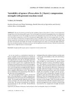
3D models were created using all the data acquired
by measuring; the models describe the influence of
stem radius and height on wood density (Fig. 4).
ere is an obvious remarkable increase in wood
density along the stem radius in all the models. In
the CW zone, the increase is more distinct in the first
40 years of growth, then the wood density stagnates. In
the other zones, i.e. OW, SWL and SWR, the increase
is constant along the entire stem radius. e remark-
able influence of the stem radius on wood density cor-
responds with the statistical results of ANOVA.
Wood density decreases in the CW zone with the
increasing height. In the side zones SWL and SWR
it is also possible to see a gradual decrease in density
with the increasing stem height. Only the model for
the OW zone shows an opposite trend. However,
looking closely at the model, we can see the values
measured at various heights are not significantly dif-
ferent. e reverse trend in this zone can be caused
by the fact the data from lower positions in the
stem are missing. To sum up, the insignificance of
the wood density changes along the stem height in
our models is again a confirmation of the statistical
results of ANOVA. e created functions and equa-
tion coefficients valid for the description of the wood
density variability in relation to the position in the
stem are shown in Table 6. e marked influence of
the position in the stem on wood density was con-
firmed by high correlation coefficients of the selected
sets (0.517 up to 0.718).

When the macroscopic and microscopic structure
changes, considerable changes in properties, in our
case in wood density, can also be expected. Fig. 5
clearly shows a trend when density increases with the
increasing percentage of compression wood in the
sample. When there is 10% of compression wood in
the total area of the sample front, the wood density
is 475 kg/m
3
, which is a value similar to the density
of standard wood. When there is 80% of compression
wood in the front, the density is 680 kg/m
3
, in other
words, it is 1.5 times higher. e created model that
describes the influence of compression wood on den-
sity was statistically significant and the high values
of correlation coefficients confirm the statistically
significant relation between the researched values.
e function describing the relation between the
density and the proportion of compression wood, the
correlation coefficients and equation coefficients are
represented in Table 5.
DISCUSSION
e change in the wood density variability along
the stem radius is often connected with the tree
age, as the cambium of older trees forms consid-
Table 5. e resulting function for the wood density model dependent on the compression wood area in the sample
Function
Coefficient of determination Coefficients

sampling basis a b
y = a + bx
2
lnx 0.55 0.54 474.52 0.0065
Table 6. e resulting functions for the wood density (w = 12%) dependent on the position in the stem
Zone Function
Coefficient of determination Coefficients
sampling basis a b c d
CW z = a + bx + cy + dy
2
0.52 0.51 592.26 –4.27 1.27 0.04
OW z = a + bx + cy + dy
2
0.72 0.71 587.23 1.12 –4.30 0.03
SWL z = a + blnx + cy 0.56 0.56 572.99 –5.99 –1.93
SWR z = a + bx + cy 0.62 0.61 565.75 –1.17 –1.77
10 30 50 70
Compression wood (%)
700
650
600
550
500
450
400
Density (kg/m
3
)
Fig. 5. e influence of compression wood on wood density
(w = 12%)

700
650
600
550
500
450
400
Density (kg/m
3
)
J. FOR. SCI., 53, 2007 (3): 129–137 135
erably narrower rings (with a high proportion of
late-wood) compared to the rings in the juvenile
wood area (R 2002; M 2000; P,
K 1961; T 1939). e
lowest density in the spruce wood is near the pith;
then the density increases in the radial direction
proportionally to the decreasing width of rings; on
the periphery, in the sapwood with narrow rings,
the density reaches its highest value (L et al.
1952). P and Z (1980) classify spruce
wood as soft wood, where the density increases in
the direction from the pith to the periphery, which
might be caused by the growing proportion of
late-wood in a ring. e authors also pointed out
to the analogy between the trends of late-wood
density and late-wood tracheid length, as both
the values grow with the stem radius, whereas the
early-wood density falls in the direction from the
pith to the mature wood and then it is constant.

M and D (1997) concentrated on
the wood of Sitka spruce (Picea sitchensis [Bong.]
Carr) and described a decrease in the density of the
rings formed first. e density decreased between
the second and the sixth ring from 450 kg/m
3
to
330 kg/m
3
. e authors explained the decrease as
a result of the increasing ring width and the larger
radial dimension of tracheids.
e created 3D models (Fig. 4), which describe
wood density in relation to the position in the stem,
also show the increase in wood density with the
stem radius. is transition can be caused both by
the decrease in the ring width along the stem radius
(G, H 2004), and also by the increasing
proportion of late-wood in the rings. Further, the
thickness of tracheid cell walls, which grows with
the increasing distance along the stem radius, can
also be expected to positively influence wood density
(Z, S 1986). e models do not show a
decrease in wood density near the pith, as presented
by M and D (1997), because the wood
near the pith was removed when the samples were
created and because the wood density change among
a few rings would be difficult to demonstrate in a
3D model.
Furthermore, considerable changes in wood den-

sity with the stem height have also been confirmed.
L et al. (1952) stated that even with the ring
width being identical, there were lower proportions
of late-wood at higher positions of the stem than at
lower positions. When the rings are wider at higher
positions than at lower positions, it is only natural
that this is manifested by a decrease in wood density.
P and K (1961) also confirmed a
decrease in wood density with the increasing stem
height. B (1974) reported the more-or-less
identical density in the spruce along the whole stem.
R (2002) did not confirm that the wood density
decreased with a higher stem.
e measurements of the sample tree proved a
very gradual decrease in wood density with the in-
creasing height in the side zones. In the CW zone,
the decrease is more than apparent and it is caused
by the presence of a well-developed compression
zone in lower parts of the stem. In the opposite
zone, the trend is reverse; however, the difference
between the lower and the upper parts of the stem
is very small.
S (1999), T (1986), S and J
(1978), S et al. (1984), K (1973), R
(1957) and others agreed that the density of com-
pression wood was considerably higher in compari-
son with opposite wood or to standard wood.
e values of compression wood density found
out in the sample tree also clearly confirm higher
density of compression wood, which is 550 kg/m

3
at
a 12% moisture content as compared to 450 kg/m
3
in
the opposite zone. e wide range of varying values
of compression wood density presented by various
authors was caused by different types and amounts
of compression wood in the researched samples.
High variability of compression wood density is
shown in Fig. 5, where the variability of compression
wood density was explored in relation to the area of
compression wood in the sample. e range of val-
ues from 500 kg/m
3
to 700 kg/m
3
is a good example.
is varying density of compression wood is caused
by the presence and the amount of thick-walled
compression tracheids whose cell wall thickness is
considerably higher (T 1986) compared to the
cell walls of early-wood and late-wood tracheids of
standard wood.
It is obvious that reaction compression wood
has a different structure from standard wood. For
a modified structure we can also expect different
wood properties. Compression wood has a differ-
ent structure that is manifested in the researched
wood property – density. When processing and

using wood where compression wood is present
it is necessary to expect some troubles. Because the
compression wood density is higher, higher ener-
gy will be needed for any work with the material;
moreover, compression wood has a different tint,
which may look improper for some products un-
less the difference is requested. To conclude, this
work was aimed and managed to expand the know-
ledge of the properties of Norway spruce (Picea
abies [L.] Karst.) wood with the presence of reac-
tion wood.
136 J. FOR. SCI., 53, 2007 (3): 129–137
R e f e r e n ces
BERNHART A., 1964. Über die Rohdichte von Fichtenholz.
Holz als Roh- und Werkstoff, 22: 215–227.
BOSSHARD H.H., 1974. Holzkunde, Band 2 Zur Biologie,
Physik und Chemie des Holzes. Basel, Stuttgart, Birkhäuser
Verlag: 312.
GINDL W., TEISCHINGER A., 2003. Comparison of the
TL-shear strength of normal and compression wood of
European larch. Holzforschung, 57: 421–426.
GRAMMEL R., 1990. Zusammenhänge zwischen Wachs-
tumsbedingungen und Holztechnologischen Eigenschaf-
ten der Fichte. Forstwissenschaftliches Centralblatt, 109:
119–129.
GRYC V., HOLAN J., 2004. Vliv polohy ve kmeni na šířku
letokruhu u smrku (Picea abies /L./ Karst.) s výskytem
reakčního dřeva. Acta Universitatis Agriculturae et Silvi-
culturae Mendelianae Brunensis, LII: 59–72.
GRYC V., HORÁČEK P., 2005. Effect of the position in a stem

on the length of tracheids in spruce (Picea abies [L.] Karst.)
with the occurrence of reaction wood. Journal of Forest
Science, 51: 203–212.
JANOTA I., KRIPEŇ J., 1960. Vlastnosti dreva jedle a smre-
ka niektorých oblastí na Slovensku. Drevársky výskum, 5:
5–21.
KOMMERT R., 1987. Zur Verteilung der Raumdichte und
Darrdichte zwischen und in Fichtenstämmen eines abtriebs-
reifen Baumholzes. Wissenschaftliche Zeitschrift der TU
Dresden, 36: 251–254.
KUČERA B., 1973. Holzfehler und ihr Einfluß auf die mecha-
nischen Eigenschaften der Fichte und Kiefer. Holztechno-
logie, 14: 9–17.
LEXA J., NEČESANÝ V., PACLT J., TESAŘOVÁ M., ŠTOFKO
J., 1952. Mechanické a fyzikální vlastnosti dreva. Bratislava,
Práca – Vydavateľstvo ROH: 432.
MERFORTH C., 2000. Formstabilität von Kanthölzern aus
Fichte (Picea abies /L./ Karst.) unter dem Einfluß wachsen-
der Holzfeuchte. [Dissertation.] Freiburg, Albert-Ludwigs
Universität: 235.
MITSCHELL M.D., DENNE M.P., 1997. Variation in density of
Picea sitchensis in relation to within-tree trends in tracheid
diameter and wall thickness. Forestry, 70: 47–60.
MOZINA I., 1960. Über die Zusammenhang zwischen Jahr-
ringbreite und Raumdichte bei Douglasie. Holz als Roh- und
Werkstoff, 18: 409–413.
NEČESANÝ V., 1955. Submikroskopická morfologie
buněčných blan reakčního dřeva jehličnatých. Biológia,
3: 647–657.
NEČESANÝ V., 1956. Struktura reakčního dřeva. Preslia,

28: 61–65.
NIEMZ P., SONDEREGGER W., 2003. Untersuchungen zur
Korrelation ausgewählter Holzeigenschaften untereinander
mit der Rohdichte unter Verwendung von 103 Holzarten.
Schweizerische Zeitschrift für Forstwesen, 154: 489–493.
PALOVIČ J., KAMENICKÝ J., 1961. Rozloženie rozhodujú-
cich fyzikálnych a mechanických vlastností v kmeni smreka
a jedle a ich vzťah k rozvoju nových smerov technológií
ihličnatých drevín. I. časť: Rozptyl a rozloženie objemovej
váhy, šírky ročných kruhov, podielu letného prírastku.
Drevársky výskum, 6: 85–101.
PANSHIN A.J., DE ZEEUW C., 1980. Textbook of Wood
Technology. Structure, Identifications, Properties, and Uses
of the Commercial Woods of the United States and Canada.
New York, McGraw-Hill, Inc.: 722.
PERSTORPER M., JOHANSSON M., KLIGER R., JOHANS-
SON G., 2001. Distortion of Norway spruce timber. Part 1.
Variation of relevant wood properties. Holz als Roh- und
Werkstoff, 59: 94–103.
PETTY J.A., MACMILLIAN D.C., STEWARD C.M., 1990.
Variation and growth ring width in stems of Sitka and
Norway spruce. Forestry, 70: 39–49.
RAK J., 1957. Fysikální vlastnosti reakčního dřeva smrku.
Drevársky výskum, 2: 27–52.
RECK P., 2002. Das Bauwachstum von kronnenspunnung-
frei gewachsenen Fichten (Picea abies (L.) Karst.) unter
besonderer Berücksichtigung der Holztechnologischen
Eigenschaften. [Dissertation.] Freiburg, Albert-Ludwigs
Universität: 260.
SEELING U., 1999. Einfluß von Richtgewebe (Druckholz) aud

Festigkeit und Elastizität des Druckholes. Holz als Roh- und
Werkstoff, 57: 81–91.
SETH M.K., JAIN K.K., 1978. Percentage of compression
wood and specific gravity in Blue pine (Pinus wallichiana
A. B. Jackson). Wood Science and Technology, 12: 17–24.
SCHULZ H., BELLMANN B., WAGNER L., 1984. Druck-
holz, Rohdichte und Wasseraufnahme. Holz als Roh- und
Werkstoff, 42: 399.
TIMELL T.E., 1986. Compression Wood in Gymnosperms,
Volume 1. Bibliography, Historical Background, Deter-
mination, Structure, Chemistry, Topochemistry, Physical
Properties, Origin and Formation of Compression Wood.
Berlin, Springer Verlag: 705.
TRENDELENBURG R., 1932. Über die Eigenschaften des Rot-
oder Druckholzes der Nadelhölzer. Allgemeine Forst- und
Jagdzeitung, 108: 1–14.
TRENDELENBURG R., 1939. Das Holz als Rohstoff. Mün-
chen, Berlin, Lehmans Verlag: 435.
WAGENFÜHR R., 1999. Anatomie des Holzes, Strukturana-
lytik – Identifiziefung – Nomenklatur – Mikrotechnologie.
Leipzig, DRW-Verlag: 188.
ZOBEL B.J., SPRAGUE J.R., 1986. Juvenile Wood in Forest
Trees. Berlin, Heidelberg, Springer-Verlag: 300.
ČSN 49 0102, 1988. Metóda zisťovania priemernej šírky
letokruhov a priemerného podielu letného dreva. Praha,
Vydavatelství Úřadu pro normalizaci a měření: 8.
Received for publication June 20, 2006
Accepted after corrections July 7, 2006
J. FOR. SCI., 53, 2007 (3): 129–137 137
Variabilita hustoty dřeva smrku (Picea abies [L.] Karst.) s přítomností

reakčního dřeva
ABSTRAKT: Studie se zabývá vyhodnocením integrální veličiny určující vlastnosti dřeva – hustoty dřeva při vlhkosti
0 % a 12 %. Hustota dřeva byla zkoumána na vzorníkovém stromě s přítomností reakčního tlakového dřeva. Hustota
dřeva byla stanovena pro jednotlivé zóny (CW, OW, SWL a SWR). Zóna s přítomností tlakového dřeva (CW) má vyšší
hustotu než zóny zbývající. Ze získaných dat byly vytvořeny 3D modely pro jednotlivé zóny, které popisují variabilitu
hustoty dřeva po poloměru a výšce kmene. Vliv poloměru se statisticky jeví jako velmi významný faktor. U zkušeb
-
ních vzorků s přítomností tlakového dřeva se hustota dřeva významně zvyšuje. Při 80% podílu tlakového dřeva ve
zkušebním vzorku byla hustota dřeva 1,5krát vyšší ve srovnání se dřevem bez přítomnosti tlakového dřeva.
Klíčová slova: smrk; hustota; tlakové dřevo
Corresponding author:
Ing. V G, Ph.D., Mendelova zemědělská a lesnická univerzita v Brně, Lesnická a dřevařská fakulta,
Lesnická 37, 613 00 Brno, Česká republika
tel.: + 420 545 134 548, fax: + 420 545 211 422, e-mail: