Báo cáo lâm nghiệp: " Comparison of three methods to determine optimal road spacing for forwarder-type logging operations" pdf

J. FOR. SCI., 55, 2009 (9): 423–431 423
JOURNAL OF FOREST SCIENCE, 55, 2009 (9): 423–431
Road network planning is an important part of
logging planning. e optimized road network can
help minimize harvesting costs. To optimize the road
network, optimum road density and spacing should
be analyzed.
In Austria, the road density is 49.1 m/ha for small
forests less than 200 ha, 41.8 m/ha for private forests,
33.27 m/ha for federal forests and average 45 m/ha
overall (www.bfw.ac.at). M (1942) de-
veloped a model to define optimum road spacing
based on minimizing the total cost of skidding and
roading from the viewpoint of a landowner. Major
variables are removals per ha, skidding cost, road
costs and landing costs. Many researchers have
used Matthews’ model. Additional factors influenc-
ing optimum road spacing (ORS) were identified by
several researchers.
Logging method, price of products, taxation
policies, landing costs, overhead costs, equipment
opportunity costs, width of road and the size of
landing, skidding pattern, profit of logging contrac-
tor, slope, topography and soil disturbance influence
ORS (S 1964; S 1976; P
1978; B 1983; W 1984; S 1986;
T 1988, 1992; Y, S 1989; L,
C 1993; H 1997; A, S-
 2001; S, B 2006).
e minimization of total cost including skidding
or forwarding cost and roading costs has been used

in previous studies (P, P 1998; N
2004). However, it is important to know what kind
of the costs should be minimized to reach the opti-
mum road spacing (ORS) and what method can be
applied to have more accurate and real results. In the
previous studies, different methods have not been
compared to introduce a more appropriate method
to study optimal road spacing. e current paper
uses three methods and compares the results.
M (1942) and S (1976) use
similar assumptions to derive their ORS formulas.
Comparison of three methods to determine optimal road
spacing for forwarder-type logging operations
M. R. G
1
, K. S
1
, J. S
2
1
Department of Forest and Soil Sciences, Institute of Forest Engineering,
University of Natural Resources and Applied Life Sciences, Vienna, Austria
2
Department of Forest Engineering, College of Forestry, Oregon State University,
Corvallis, USA

ABSTRACT: Optimum road spacing (ORS) of forwarding operation in Styria in Southern Austria is studied in this
paper. In a harvesting operation it is important to compute the ORS to minimize the total cost of harvesting and roading.
e aim of this study was a comparison of different methods to study ORS. Data from 82 cycles were used to develop
two models for predicting the cycle time using statistical analysis of a time study data base. e ORS was computed

by three methods including Matthews’ formula (1942), Sundberg’s method (1976), and the two statistical models for
predicting the cycle time. e results gave the ORS for one-way forwarding using Matthew’s formula as 1,969 m, Sund-
berg’s model as 394.4 m, and the two time study models as 463 and 909 m. e analysis of forwarding data indicated
that the speed was related to a distance which contributed to the difference between models and that the loading and
unloading time may be related to one or several other study variables.
Keywords: forwarding; production; cost; travelling model; optimum road spacing
424 J. FOR. SCI., 55, 2009 (9): 423–431
ese assumptions include constant €/m
3
/m cost
and an even distribution of logs over the harvest
area. For these assumptions, the average forwarding
cost occurs at the average forwarding distance. is
paper studies how optimum road spacing varies if
forwarding cost (including travelling, loading and
unloading cost) or travelling costs (without loading
and unloading cost) are used in the calculation us-
ing observations from a forwarding study in Austria.
Speed as a function of distance is examined. e op-
timal road spacing is also calculated using Matthews’
and Sundberg’s methods to see how road spacing
would differ depending on the study method.
METHOD OF STUDY
Study area
e production of Ponsse Buffalo Dual (A-
 2005) and Gremo 950 R cable forwarder
(W 2006) was studied in Styria in South-
ern Austria. e description of stands is presented in
Table 1. Mean harvesting volume was about 100 m
3

per ha with a mean dbh of 25 cm. e roading cost
averaged at 20 €/m.
Time prediction models
Two forwarding time prediction models are de-
veloped from data collected. e first, referred to as
the forwarding model. e second, referred to as the
travelling model, is introduced in this paper.
Forwarding model
G et al. (2006) used the collected time
study data base and developed the general model to
predict the forwarding time.
T (min/cycle) = 81.293 – 47.886 × piece volume
(m
3
) – 46.795 × type of forwarder + 0.076 × forward-
ing distance (m) – 1.189 × slope (%)
R
2
= 0.32, adjusted R
2
= 0.284, number of observa-
tions = 82.
e value for Ponsse forwarder is 1 and the value
of 0 is considered for Gremo forwarder.
R
2
= 0.949, adjusted R
2
= 0.947, number of observa-
tions = 82.

Travelling model
Stepwise regression method was applied to de-
velop this model. Travel time including travel loaded
Table 1. Description of study sites
First site Second site
Stand area (ha) 2.27 1.83
Slope (%) 11 39
Stand age (years) 70–130 90
Pre-harvest stand density (n/ha) 1,089 729
Pre-harvest standing volume (without bark) (m
3
/ha) 510.4 646
Number of harvested trees (n) 1,073 470
Total harvesting volume (m
3
) 331.8 513
Tree volume (m
3
) 0.31 0.7
Harvesting percent (%) 28.7 45
Number of trails 15 5
Length of trails (m) 40–200
190–235
Time of harvesting spring spring
Table 2. Table of the analysis of variance
Sum of squares df Mean square F Significance
Regression 9,381.36 2 4,690.68 233.4 < 0.0001
Residual 1,607.81 82 20.09
Total 10,989 84
J. FOR. SCI., 55, 2009 (9): 423–431 425

and travel empty was used as a function of the
variables such as forwarding distance, load volume,
slope, forwarding distance × load volume and slope
× load volume.
Road spacing
To study the optimum road spacing, we will apply
three methods. The first was presented by M-
 (1942) and later modified by D
(1983); A and M (1993) applied
this method to study ORS for manual skidding
of sulkies in Tanzania. The second method was
introduced by S (1976) and applied by
H (1978). Both Matthews’ and Sundberg’s
formulas are based on the minimization of costs
and assumptions of constant €/m
3
/m and that
logs are evenly distributed over the area. Constant
speed and load satisfy the assumptions of constant
€/m
3
/m.
0
5
10
15
20
25
30
35

40
45
0 50 100 150 200 250 300
Forwarding distance (m)
Speed (m/minutes)
Fig. 1. Speed for different distances from
the forwarding time study
0
5
10
15
20
25
30
35
40
0 50 100 150 200 250 300
Forwarding distance (m)
Load vomue (m
3
)
0
5
10
15
20
25
30
35
40

0 50 100 150 200 250 300
Forwarding distance (m)
Slope (%)
Fig. 2. Distribution of logs along the for-
warding distance
Fig. 3. Distribution of the slope of trail
along the forwarding distance
)
Forwarding distance (m)
Load volume (m
3
)
426 J. FOR. SCI., 55, 2009 (9): 423–431
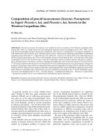
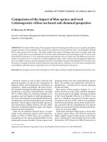
Using the travelling time and travelling distance of
time study data base, the velocity was computed for
different distances (Fig. 1).
Fig. 1 illustrates that speed is not constant and
increases with forwarding distance in this study.
Naturally, machines move faster in a longer distance
because of the time spent to accelerate and deceler-
ate. However, the difference between speeds in short
distance and long distance seems too high in this
case study. e divergences are caused by the low
load volume and gentle slope in longer distances
during the studied operations (Figs. 2 and 3).
In third and fourth method, the roading cost per
cubic meter is based on roading cost and harvest-
ing volume per ha. e forwarding and travelling
costs/m
3

also are determined by using forwarding
time, travelling time and constant hourly machine
cost regardless of the load or speed. en the sum
of roading cost and forwarding cost was plotted as
a function of road spacing. e sum of roading cost
and travelling cost was also determined and plotted
for different road spacings.
e average road construction and maintenance cost
in the study area were 16.5 and 3.5 €/m, respectively.
e harvested volume averaged at 100 m
3
per ha.
Matthews’ formula and Sundberg’s formula
Equation (1) developed by M (1942) is
used. e equation assumes that the road will not be
used for more than one year and all the logs will be
forwarded or skidded directly to the roadside.

40,000 × C
road
S =
√
––––––––––––––– (1)

V × C
travel
where:
S – optimal road spacing (m),
C
road

– cost of the construction and maintenance of 1 m road
length (€/m),
C
travel
– cost of travelling of 1 m
3
of logs to 1 m distance
(€/m
3
/m),
V – stand volume density (m
3
/ha).
Matthew’s equation can be adapted by introducing
Segebaden’s network correction factor C
net
(H-
 1997). e formula becomes as:

40,000 × C
road
× C
net
S =
√
–––––––––––––––––––––– (2)

V × C
travel
e formula can be rewritten as follows

40,000 C
road
× (4 C
net
)
S =
√
–––––––––––––––––––––– (3)

V × C
travel
Therefore the correction factor consists of a
constant of 4 and the network correction factor as
C
net
. e network correction factor is computed by
dividing the effective mean forwarding distance by
the geometric mean distance. Its value ranges from
1 to 2 (S 1964).
S (1976) specified the forwarding cost
more precisely as

c × t × (1 + p)
C
travel
= –––––––––––– (4)

L
vol

where:
c – operation of an extraction machine (€/min),
t – time consumption for the extraction cycle (min/m),
p – winding factor (0 for perpendicular off-road transport);
a correction factor designed to allow for cases where
skidding or forwarding trails are winding and not
always end at the nearest point of the road and lying
normally between the limits 0 and 0.50,
L
vol
– load volume (m
3
).
It also assumes that the €/m
3
/m is constant and the
logs are distributed evenly over the area. Substitution
of C
forw
in formula 3 results in

10,000 C
road
× L
vol
× (4 C
net
)
S =
√

–––––––––––––––––––––– (5)

V × c × t × (1 + p)
e formulas of M (1942) and S-
 (1976) are used as the first method to derive
optimal road spacing.
In the other two procedures, the roading cost per
m
3
was calculated for different road spacings using
road density, roading cost per m, harvesting volume
per ha, and the regression of cycle time. e travel-
ling cost per m
3
was calculated using hourly cost and
time prediction model assuming the load volume
and slope at their average.
e total cost was calculated by adding up roading
and travelling costs. e total cost was plotted as a
function of road spacing (Fig. 2).
RESULTS
The observed production of forwarding was
17.9 m
3
/PSH
0
(productive system hour) and the
mean load per trip was 10.04 m
3
. Using the system

cost of 120 €/hour, the forwarding cost is estimated
at about 6.72 €/m
3
.
Travelling model
e average travelling time was 9.98 min consider-
ing the mean load of 10.04 m
3
per trip, the average
production rate for travelling is 60.36 m
3
/PSH
0
. e
travelling cost would be 1.99 €/m
3
.
e stepwise regression method was used to de-
velop a travelling time prediction model. Slope of
J. FOR. SCI., 55, 2009 (9): 423–431 427
trail, forwarding distance and load volume were used
in the model.
T (min/cycle) = 0.00197 × travelling distance (m)
× load volume (m
3
) + 0.37906 × slope (%)
R
2
= 0.854, adjusted R
2

= 0.85, number of observa-
tions = 82.
e significance level of the ANOVA table con-
firms that the model makes sense at α = 0.05.
According to the travelling model, if forwarding
distance, load volume and slope increase, travelling
time will also increase.
Table 3 presents the summary statistics of meas-
urements in the time studies.
Road spacing
ere are three ways of representing the forward-
ing cost:

c × t × D c × a
0
c × b × F
C
forwding
= –––––––– + –––––––– – ––––––––– –

60 × L
vol
60 × L
vol
60 × L
vol

c × e × P c × f × S
– –––––––– – –––––––––– (6)

60 × L
vol
60 × L
vol

c × t × D × L
vol
c × d × S
C
travel
= ––––––––––––– + –––––––––– (7)

60 × L
vol
60 × L
vol
where:
D – forwarding distance (m),
L
vol
– load volume (m
3
),
F – forwarder type,
P – piece volume (m
3
),
S – slope of skid trail (%).
Equations (6) and (7) are presented based on the
forwarding and travelling model, respectively. To get

the optimal road spacing, the first derivation of the
forwarding cost function enters into further analysis,
resulting in the following equations:

c × t
C´
forw
= ––––––– (8)

240 × L
vol

c × t
C´
travel
= ––––––– (9)

240
Matthews’ formula
Two-way forwarding
To calculate the travelling cost, the average trav-
elling time of 9.98 min per cycle for an average
forwarding distance of 96.64 m was used. e time
of extraction per m distance was 0.1033 min for
favourable trail conditions. Using the hourly cost of
2 €/min, the travelling cost would be 0.00086 €/m
3
/m
based on formula (9).
If machines work in an unfavourable and steep

terrain, the estimated variable time or cost should
be increased to reflect the additional time to go the
equivalent direct distance. For example, if it is ex-
pected that the forwarder must travel 1.2 km to go
1 km, then the travel cost per direct distance is in-
creased by 20% (M 1942), i.e. from 0.00086
to 0.00103 €/m
3
/m.
e calculations yielded the optimal road spac-
ing for two-way and one-way forwarding using
Matthew’s formula of 2,784 m and 1,969 m respec-
tively.
Sundberg’s formula
Considering C
net
of 1 and p of 0.25 as average
value and input, the other variables in the formula
for ORS would be computed. e mean travel time
was 9.98 min for the average travelling distance of
96.64 m. erefore the time to travel 1 m loaded and
light would be 0.103 min. Considering C
net
of 1 for
Table 3. Summary statistics of the parameters
Parameter Max. Mean Min.
Loading (min) 42.24 17.23 2.78
Loaded travel (min) 10.72 4.22 0.35
Unloading (min) 15.31 6.50 0.97
Travel empty (min) 18.67 5.76 0.40

Cycle time (min) 57.68 33.72 8.90
Distance (m) 280.00 96.64 4.00
Slope (%) 40.00 21.62 5.00
Load volume (m
3
) 18.70 10.04 1.37
Piece volume (m
3
) 0.49 0.14 0.04
428 J. FOR. SCI., 55, 2009 (9): 423–431
two-way forwarding, Sundberg’s formula yields the
optimal road spacing of 557.7 m. For one-way forward-
ing, the optimal road spacing would be 394.4 m.
Minimization of total costs
For different road spacings, roading cost, travelling
cost, forwarding cost and total cost per cubic meter
were plotted using a created Excel worksheet.
e existing forest road density in Styria is about
49.3 m/ha. Considering the average forwarding
distance of 125 m of forwarding operation sites in
Styria, K (correction factor) may be evaluated as 6.16
by the following formula (FAO 1974):

K
Dist = –––– (10)

RD
where:
Dist – average extraction distance (km),
RD – road density (m/ha),

K – terrain factor.
Road spacing was evaluated from this formula:

10,000
Road spacing (m) = ––––––––––––––––––– (11)

Road density (m/ha)
ORS using forwarding model
In this case, the forwarding model was used to plot
the total forwarding and roading cost per m
3
for dif-
ferent road spacings (Fig. 4).
Based on the calculation, the minimum total cost
is 13.84 €/m
3
and the corresponding road spacing is
463 m. In other words, if one-way forwarding is ap
-
plied, the ORS would be 463 m. e optimal road den-
sity and average forwarding distance are 21.6 m per

ha and 285 m, respectively.
ORS using travelling model
In this method, it is assumed that the loading and
unloading time are constant. To verify this assumption,
the scatter of loading and unloading time for different
forwarding distances are plotted (Fig. 5). ere is a
weak correlation (0.47) and also very weak R
2

(0.26) for
the model, which can verify the assumption.
e average time for the sum of loading and un-
loading was 23.73 min. e production of loading
and unloading averaged at 25.38 m
3
/h with the cost
of 4.73 €/m
3
. e travel loaded and travel empty time
are dependent on road spacing, slope and load vol-
ume. e travelling time prediction model was used
to plot the total cost of travelling and roading costs
per m
3
for the range of road spacings (Fig. 6).
e minimum total cost of travelling and roading
is 6.04 €/m
3
and its corresponding road spacing is
about 909 m, which is an optimum spacing. e
optimal road density and forwarding distance are
11 m/ha and 560 m, respectively.
It should be noted that the maximum forwarding
distance was 280 m in the time study, but the optimal
forwarding distance of 560 m is higher and out of
range of the collected data base. e regression model
applied here can be improved by using further time
studies including travelling costs at distances longer
than 560 m or more to have more accurate results.

0
10
20
30
40
50
60
70
80
0 50 100 150 200 250 300 350 400 450 500
Road Spacing (m)
Cost (Euro/m^3)
Forwarding cost (Euro/m^3)
Road cost (Euro/m^3)
Total cost (Euro/m^3)
Fig. 4. e total cost summary and road spacing for one-way forwarding using the forwarding model
Forwarding cost (/m
3
)
Road cost (/m
3
)
Total cost (/m
3
)
Cost (/m
3
)
Road spacing (m)
J. FOR. SCI., 55, 2009 (9): 423–431 429

DISCUSSION
Based on Matthews’ formula, ORS for one-way
forwarding is about 1,969 m. For Sundberg’s formula,
ORS would be 394.4 m for one-way forwarding. Both
Matthews and Sundberg use assumptions of con-
stant €/m
3
/m. ey differ in how they adjust for the
terrain. Sundberg provides several explicit factors of
adjusting for the terrain.
e method of total cost minimization to study
ORS allows engineers to see the sensitivity of road-
ing, forwarding and total costs to different ORS. If the
forwarding model is used in the calculation, the ORS
for one-way forwarding would be 463 m. But if the
travelling model (similar to Matthews’ method and
Sundberg’s formula) is used, the ORS of 909 m for
one-way forwarding is yielded. e forwarding model
included loading and unloading time, the travelling
model did not. e difference in results between the
forwarding and travelling models suggests that loading
and unloading time may be related to other variables.
For example, loading time varied from a minimum
of 2.78 min to a maximum of 42.24 min (Table 3). If
the travelling model is used, under assumption that
loading and unloading times are independent of road
spacing, harvesting cost is lower as compared to the
forwarding model and this resulted in a greater ORS.
ere is a large difference between ORS (463 m and
909 m) because of the additional loading and unload-

ing cost considered in the forwarding model which
shifts the total cost line upward.
Fig. 1 shows that an increasing speed was associ-
ated with increasing forwarding distance. Since the
speed is not constant for different distances, Mat-
thews’ and Sundberg’s formulas would not be the
appropriate methods to study ORS in this case study.
y = 3.6452Ln(x ) + 9.2284
R
2
= 0.2654
0
10
20
30
40
50
60
0 50 100 150 200 250 300
Forwarding distance (m)
Loading and unloading time
Fig. 5. Scatter of loading and
unloading time with forwarding
distance
0
2
4
6
8
10

12
14
16
18
20
22
24
0 200 400 600 800 1,000 1,200
Road spacing (m)
Costs (Euro/m
3
)
Traveling cost (Euro/m^3)
Road cost (Euro/m^3)
Total cost (Euro/m^3)
Fig. 6. e total cost, travelling cost and roading cost for different road spacings for one-way forwarding using the travelling
model
Travelling cost (/m
3
)
Road cost (/m
3
)
Total cost (/m
3
)
Cost (/m
3
)
Road spacing (m)

y = 3.6452Ln(x) + 9.2284
R
2
= 0.2654
430 J. FOR. SCI., 55, 2009 (9): 423–431
Of course, both Matthews’ and Sundberg’s formulas
could be respecified if the speed was specified as a
function of distance.
Although the cycle time equations are appropri-
ate for this study, the ORS values derived from the
case study cannot be applied to other areas unless
they have the same non-uniform conditions along
the trail. In this case study, the non-uniform condi-
tions were smaller loads and flatter slopes at longer
forwarding distances.
e computed optimal road density is lower than the
current road density in Austria because 48.3% of the
forest land is owned by small private forest owners. It
is also lower than the road density in the federal forests.
e results of this study would be applicable to the
areas with similar terrain and forest removals.
CONCLUSIONS
Optimal road spacing is an important factor in
logging planning to help minimizing the total cost of
harvesting and roading. e comparisons of different
available methods to get optimum road spacing can
be useful for planners to choose the most appropri-
ate method based on their local conditions.
Acknowledgement
e authors appreciate Prof. Dr. H from

ETH Zurich for his valuable review comments used
in this article.
R ef ere nc e s
ABELLI
W.S., MAGOMU G.M., 1963. Optimal road spacing
for manual skidding sulkies. Journal of Tropical Forest
Science, 6: 8–15.
AFFENZELLER G., 2005. Integrierte Harvester-Forwarder-
Konzepte Harwarder. [MSc esis.] Vienna, University of
Natural Resources and Applied Life Sciences, Institute of
Forest Engineering: 63.
AKAY A., SESSIONS J., 2001. Minimizing road construction
plus forwarding costs under a maximum soil disturbance
constraint. In: e International Mountain Logging and
11
th
Pacific Northwest Skyline Symposium, December
10–12, Seattle. Washington, D.C.: 268–279.
BRYER J.B., 1983. e effects of a geometric redefinition of the
classical road and landing spacing model through shifting.
Journal of Forest Science, 29: 670–674.
DYKSTRA D.P., 1983. Fundamentals of forest road design and
layout. Stencil No. EFn 7. Morogoro, University of Dar es
Salaam, Division of Forestry: 28.
FAO, 1974. Logging and Log Transport in Tropical High For-
est. Rome, FAO: 50–52.
GHAFFARIAN M.R., STAMPFER K., SESSIONS J., 2007.
Forwarding productivity in Southern Austria. Croatian
Journal of Forest Engineering, 28: 169–175.
HEINIMANN H.R., 1997. A computer model to differentiate

skidder and cable-yarder based road network concepts on
steep slopes. Journal of Forest Research (Japan), 3: 1–9.
HEINIMANN H.R., 2002. Erschliessungsplanung im laend-
lichen Raum. Class Notes. Zurich, ETH: 73.
HUGGARD E.R., 1978. Optimum road spacing. Quarterly
Journal of Forestry, 72: 207–210.
LIU S., CORCORAN T.J., 1993. Road and landing spacing
under the consideration of surface dimension of road and
landings. International Journal of Forest Engineering, 5:
49–53.
MATTHEWS D.M., 1942. Cost Control in the Logging In-
dustry. New York, McGraw-Hill: 374.
NAGHDI R., 2004. Study of optimum road density in tree
length and cut to length system. [PhD Thesis.] University
of Tarbiat Modarres, Faculty of Natural Resources: 152.
PETERS P.A., 1978. Spacing of roads and landings to mini-
mize timber harvest cost. Journal of Forest Science, 24:
209–217.
PICMAN D., PENTEK T., 1998. e influence of forest roads
building and maintenance costs on their optimum density
in low lying forests of Croatia. In: Seminar on Environmen-
tally Sound Forest Roads and Wood Transport in Sinaia,
Romania. Rome, FAO: 87–102.
SEGEBADEN G.V., 1964. Studies of cross-country transpor-
tation distances and road net extension. Studia Forestalia
Suecica, No. 18: 70.
SESSIONS J., 1986. Can income tax rules affect management
strategies for forest roads. Western Journal of Applied
Forestry, 1: 26–28.
SESSIONS J., BOSTON K., 2006. Optimization of road spac-

ing for log length shovel logging on gentle terrain. Interna-
tional Journal of Forest Engineering, 17: 67–75.
SUNDBERG U., 1976. Harvesting Man-made Forests in De-
veloping Countries. Rome, FAO: 185.
THOMPSON M.A., 1988. Optimizing spur road spacing on the
basis of profit potential. Forest Product Journal, 38: 53–57.
THOMPSON M.A., 1992. Considering overhead costs in road
and landing spacing models. International Journal of Forest
Engineering, 3: 13–19.
WENGER K., 1984. Cost Control Formulas for Logging Op-
erations. 2
nd
Ed. Society of American Foresters. New York,
John Wiley and Sons: 1335.
WRATSCHKO B., 2006. Einsatsmöglichkeiten von Seil-
forwarded. [MSc esis.] Vienna, University of Natural
Resources and Applied Life Sciences, Institute of Forest
Engineering: 66.
J. FOR. SCI., 55, 2009 (9): 423–431 431
Corresponding author:
M R G, University of Natural Resources and Applied Life Sciences,
Institute of Forest Engineering, Department of Forest and Soil Sciences, Peter-Jordan Strasse 82/3, A-1190 Vienna, Austria
tel.: + 43 147 654 43 06, fax: + 43 147 654 43 42, e-mail:
Porovnání tří metod k určení optimálního rozestupu lesních cest
pro těžební operace s vyvážením dříví forwarderem
ABSTRAKT: V práci byly studovány optimální rozestupy lesních cest pro vyvážení dříví ve Štýrsku (jižní Rakousko).
Při těžebních operacích je důležité vypočítat optimální rozestup cest tak, aby se minimalizovaly celkové náklady na
těžbu a soustřeďování. Cílem studie bylo porovnání různých metod používaných k určení optimálního rozestupu
cest. Data z 82 cyklů byla použita pro vytvoření dvou modelů sloužících k predikci času na jeden cyklus za použití
báze časoměrných dat. Optimální rozestup cest byl vypočítán pomocí tří metod včetně rovnice podle Matthewse

(1942), Sundbergovy metody (1976) a dvou statistických modelů pro predikci doby cyklu. Výsledky ukázaly, že podle
Matthewse byl optimální rozestup cest pro jednosměrné vyvážení 1 969 m, podle Sundbergova modelu 394,4 m
a podle dvou modelů časové studie 463 a 909 m. Analýza dopravních dat ukázala souvislost mezi rychlostí a vzdá
-
leností, která přispěla k rozdílům mezi modely, a to, že čas pro nakládku a vykládku mohl být ve vztahu s jednou či
více studovanými proměnnými.
Klíčová slova: vyvážení; výnosy; náklady; dopravní model; optimální rozestup cest
YEAP Y.H., SESSIONS J., 1988. Optimizing road spacing and
road standards simultaneously on uniform terrain. Journal
of Tropical Forest Science, 1: 215–228.
http:// www.bfw.ac.at
Received for publication September 18, 2008
Accepted after corrections April 17, 2009