.Ocean Modelling for Beginners Phần 4 pptx

44 3 Basics of Geophysical Fluid Dynamics
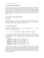
Fig. 3.12 Appearance of straight path (white line) of an object (ball) for an observer on a rotating
turntable. The inner end of the white line shows the starting position of the object. The SciLab
script “Straight Path.sce” in the folder “Miscellaneous/Coriolis Force” of the CD-ROM produces
an animation
3.12.2 The Centripetal Force and the Centrifugal Force
Consider an object attached to the end of a rope and spinning around with a rotating
turntable. In the f xed coordinate system, the object’s path is a circle (Fig. 3.13) and
the force that deflect the object from a straight path is called the centripetal force.
This force is directed toward the centre of rotation (parallel to the rope) and, hence,
Fig. 3.13 Left panel In the f xed frame of reference, an object attached to a rope and rotating
at the same rate as the turntable experiences only the centripetal force. Right panel: The object
appears stationary in the rotating frame of reference, which implies a balance between the cen-
tripetal force and the centrifugal force. The SciLab script “Centripetal Force.sce” in the folder
“Miscellaneous/Coriolis Force” of the CD-ROM produces an animation
3.12 The Coriolis Force 45
operates perpendicular to the object’s direction of motion. The centripetal force (per
unit mass), which is a true force, is given by:
Centripetal force =−Ω
2
r (3.31)
where r is the object’s distance from the centre of the turntable, and Ω = 2π/T
is the rotation rate with T being the rotation period. Per definition the rotation rate
Ω is positive for anticlockwise rotation and negative for clockwise rotation. When
releasing the object, it will fl away on a straight path with reference to the f xed
frame of reference.
In the rotating frame of reference, on the other hand, the object remains at the
same location and is therefore not moving at all. Consequently, the centripetal force
must be balanced by another force of the same magnitude but acting in the opposite
direction. This apparent force – the centrifugal force – is directed away from the
centre of rotation. Accordingly, the centrifugal force is given by:

Centrifugal force =+Ω
2
r (3.32)
When releasing the object, an observer in the rotating frame of reference will see
the object flyin away on a curved path – similar to that shown in Fig. 3.12.
3.12.3 Derivation of the Centripetal Force
The speed of any object attached to the turntable is the distance travelled over a time
span. Paths are circles with a circumference of 2πr, where r is the distance from the
centre of rotation, and the time span to complete this circle is the rotation period.
Accordingly, the speed of motion is given by:
v =
2π
T
r = Ωr. (3.33)
During rotation, the speed of parcels remains the same, but the direction of
motion and thus the velocity changes (Fig. 3.14). The similar triangles in Fig. 3.14
give the relation δv/v = δL/r. Since δL is given by speed multiplied by time span,
this relation can be rearranged to yield the centripetal force (per unit mass):
dv
dt
=−
v
2
r
, (3.34)
where the minus sign has been included since this force points toward the centre of
rotation. Equation (3.31) follows, if we finall insert (3.33) into the latter equation.
46 3 Basics of Geophysical Fluid Dynamics
Fig. 3.14 Changes of location and velocity of a parcel on a turntable
3.12.4 The Centrifugal Force in a Rotating Fluid

Consider a circular tank fille with flui on a rotating turntable. Letting the tank
rotate at a constant rate for a long time, all flui will eventually rotate at the same
rate as the tank. In this steady-state situation, the flui surface attains a noneven
shape, as sketched in Fig. 3.15. The fina shape of the flui surface is determined by
a balance between the centrifugal force and a centripetal force, that, in our rotating
fluid is provided by a horizontal pressure-gradient force provided by a slanting flui
surface. This balance of forces reads:
− g
∂η
∂r
=−Ω
2
r (3.35)
where r is the radial distance from the centre of the tank.
The analytical solution of the latter equation is:
η(r) =
1
2
Ω
2
g
r
2
−η
o
, (3.36)
Fig. 3.15 Sketch of the steady-state force balance between centrifugal force (CF) and pressure-
gradient force (PGF) in a rotating f uid. The dashed line shows the equilibrium surface level for
the nonrotating case
3.12 The Coriolis Force 47

where the constant η
o
can be determined from the requirement that the total volume
of flui contained in the tank has to be conserved (if the tank is void of leaks). The
tank’s rotation leads to a parabolic shape of the flui surface and it is essentially
gravity (via the hydrostatic balance) that operates to balance out the centrifugal
force. The latter balance is valid for all flui parcels in the tank. The pathways of
flui parcels are circles in the fi ed frame of reference. The observer in the rotating
system, however, will not spot any movement at all.
3.12.5 Motion in a Rotating Fluid as Seen in the Fixed Frame
of Reference
With reference to a f xed frame of reference, flui parcels in the rotating tank
exclusively feel the centripetal force provided by the pressure-gradient force. In
the absence of relative motion, flui parcels describe circular paths. How does the
trajectory of a flui parcel look like, if we give it initially a push of a certain
speed into a certain direction? The momentum equations governing this problem are
given by:
dU
dt
=−Ω
2
X and
dV
dt
=−Ω
2
Y (3.37)
where (X, Y) refers to a location and (U, V ) to a velocity in the f xed coordi-
nate system. On the other hand, the location of our flui parcel simply changes
according to:

dX
dt
= U and
dY
dt
= V (3.38)
Owing to rotation, velocities in the fi ed and rotating reference systems are not
the same. Instead of this, it can be shown that they are related according to:
U = u −Ω y and V = v +Ω x (3.39)
where (x, y) refers to a location and (u,v) to a velocity in the rotating coordinate
system.
3.12.6 Parcel Trajectory
Before reviewing the analytical solution, we employ a numerical code (see below)
to predict the pathway of a flui parcel in a rotating flui tank as appearing in the
fi ed frame of reference. To this end, we consider a flui tank, 20 km in diameter,
rotating at a rate of Ω = −0.727×10
−5
s
−1
, which corresponds to clockwise rotation
with a period of 24 h.
48 3 Basics of Geophysical Fluid Dynamics
At location X = x = 0 and Y = y = 5 km, a disturbance is introduced such that
the flui parcel obtains a relative speed of u
o
= 0.5 m/s and v
o
= 0.5 m/s. In the f xed
coordinate frame, the initial velocity is U
o

= 0.864 m/s and V
o
=0.5m/s.
The results show that the resultant path of the flui parcel is elliptical (Fig. 3.16).
With a closer inspection of selected snapshots of the animation (Fig. 3.17), we can
also see that the flui parcel comes closest to the rim of the tank twice during
one full revolution of the flui tank. This finding which is simply the result of
the elliptical path, is the important clue to understand why so-called inertial oscilla-
tions, described below, have periods half that associated with the rotating coordinate
system.
Fig. 3.16 Trajectory of motion (white line) for one complete revolution of a clockwise rotating
flui tank as seen in the f xed frame of reference. The SciLab script “Traject” in the folder “Mis-
cellaneous/Coriolis Force” of the CD-ROM produces an animation
Fig. 3.17 Same as Fig. 3.16, but shown for different time instances of the simulation. The tank
rotates in a clockwise sense. The star denotes a f xed location at the rim of the rotation tank
3.12.7 Numerical Code
In finite-di ference form, the momentum equations (3.37) can be written as:
U
n+1
= U
n
−Δt ·Ω
2
X
n
and V
n+1
= V
n
−Δt ·Ω

2
Y
n
(3.40)
3.12 The Coriolis Force 49
where n is time level and Δt is time step. The trajectory of our flui parcel can be
predicted with:
X
n+1
= X
n
+Δt ·U
n+1
and Y
n+1
= Y
n
+Δt · V
n+1
(3.41)
Again, predictions from the momentum equations are inserted into the latter
equations as to yield an update of the locations. I decided to tackle this problem
entirely with SciLab without writing a FORTRAN simulation code.
3.12.8 Analytical Solution
Equations (3.37) and (3.38) can be combined to yield:
d
2
X
dt
2

=−Ω
2
X and
d
2
Y
dt
2
=−Ω
2
Y (3.42)
The solution of these equations that satisfie initial conditions in terms of location
and velocity are given by:
X(t) = X
o
cos(Ωt) +
U
o
Ω
sin(Ωt) (3.43)
Y (t) = Y
o
cos(Ωt) +
V
o
Ω
sin(Ωt) (3.44)
This solution describes the trajectory of a parcel along an elliptical path. In the
absence of an initial disturbance (u = 0 and v = 0), and using (3.39), the latter
equations turn into:

X(t) = X
o
cos(Ωt) −Y
o
sin(Ωt)
Y (t) = Y
o
cos(Ωt) + X
o
sin(Ωt)
which is the trajectory along a circle of radius

X
2
o
+Y
2
o
, as expected.
3.12.9 The Coriolis Force
We can now reveal the Coriolis force by translating the trajectory seen in the f xed
frame of reference (see Fig. 3.16), described by (3.43) and (3.44), into coordinates
of the rotating frame of reference. The corresponding transformation reads:
x = X cos(Ωt) +Y sin(Ωt) (3.45)
y = Y cos(Ωt) − X sin(Ωt). (3.46)
Figure 3.18 shows the resultant fl w path as seen by an observer in the rotating frame
of reference. Interestingly, the flui parcel follows a circular path and completes the
50 3 Basics of Geophysical Fluid Dynamics
Fig. 3.18 Pathway of an object that experiences the Coriolis force in a clockwise rotating f uid.
The SciLab script “Coriolis Force Revealed.sce” in the folder “Miscellaneous/Coriolis Force” of

the CD-ROM produces an animation
circle twice while the tank revolves only once about its centre. Accordingly, the
period of this so-called inertial oscillation is 0.5 T , known as inertial period, with
T being the rotation period of the flui tank.
Rather than working in a fi ed coordinate system, it is more convenient to for-
mulate the Coriolis force from the viewpoint of an observer in the rotating frame of
reference. In the absence of other forces, it can be shown that inertial oscillations
are governed by the momentum equations:
∂u
∂t
=+2Ω v and
∂v
∂t
=−2Ω u (3.47)
The Coriolis force acts perpendicular to the direction of motion and the factor
of 2 reflect the fact that inertial oscillations have a period half that of the rotating
frame of reference. If a parcel is pushed with an initial speed of u
o
into a certain
direction, it can also be shown that its resultant path is a circle of radius u
o
/(2
|
Ω)
|
).
With an initial speed of about 0.7 m/s and
|
Ω
|

= 0.727×10
−5
s
−1
, as in the above
example, this inertial radius is about 4.8 km.
3.13 The Coriolis Force on Earth
3.13.1 The Local Vertical
In rotating fluid at rest, the centrifugal force is compensated by pressure-gradient
forces associated with slight modificatio of the shape of the flui surface. On the
rotating Earth, this leads to a minor variation of the gravity force by less than 0.4%.
The local vertical at any geographical location is now define as the coordinate
axis aligned at right angle to the equilibrium sea surface. This implies that, for a
3.13 The Coriolis Force on Earth 51
Fig. 3.19 Balances of forces on a rotating Earth fully covered with seawater in a state at rest. The
gravity force (GF) is directed toward the Earth’s centre. The centrifugal force (CF) acts perpendic-
ular to the rotation axis. The pressure-gradient force (PGF) balances the combined effects of GF
and CF. The local vertical is parallel to PGF
state at rest, the pressure-gradient force along this local vertical perfectly balances
the combined effect of the gravity force and the centrifugal force (Fig. 3.19).
3.13.2 The Coriolis Parameter
Owing to a discrepancy between the orientations of the rotation axis of Earth and
the local vertical, the magnitude of the Coriolis force becomes dependent on geo-
graphical latitude and Eqs. (3.47) turn into:
∂u
∂t
=+f v and
∂v
∂t
=−fu (3.48)

where f = 2Ω sin(ϕ), with ϕ being geographical latitude, is called the Coriolis
parameter. The Coriolis parameter changes sign between the northern and southern
hemisphere and vanishes at the equator. This variation of the Coriolis parameter can
be explained by a modificatio of the centripetal force in dependence of the orienta-
tion of the local vertical (Fig. 3.20). Consequently, the period of inertial oscillations
is T = 2π/
|
f
|
and it depends exclusively on geographical latitude. It is 12 hours at
the poles and goes to infinit near the equator. The radius of inertial circles is given
by u
o
/
|
f
|
. Inertial oscillations attain a clockwise sense of rotation in the northern
hemisphere and describe counterclockwise paths in the southern hemisphere.
52 3 Basics of Geophysical Fluid Dynamics
Fig. 3.20 The centripetal force for a variation of the orientation of local vertical
3.13.3 The f -Plane Approximation
The curvature of the Earth’s surface can be ignored on spatial scales of 100 km, to
first-orde approximation. Hence, on this scale, we can place our Cartesian coordi-
nate system somewhere at the sea surface with the z-axis pointing into the direction
of the local vertical and use a constant Coriolis parameter (Fig. 3.21). The constant
value of f is define with respect to the point-of-origin of our coordinate system.
This configuratio is called the f-plane approximation.
3.13.4 The Beta-Plane Approximation
The curved nature of the sea surface can still be ignored on spatial scales of up to

a 1000 km (spans about 10
◦
in latitude), if the Coriolis parameter is described by a
constant value plus a linear change according to:
f = f
o
+β y (3.49)
Fig. 3.21 The sketch gives an example of a f-plane. The Coriolis parameter is given by
f = 2Ω sin(ϕ), where ϕ is geographical latitude of the centre of the plane
3.14 Exercise 4: The Coriolis Force in Action 53
In this approximation, β is the meridional variation of the Coriolis parameter
with a value of β = 2.2 × 10
−11
m
−1
s
−1
at mid-latitudes, and y is the distance in
metres with respect to the centre of the Cartesian coordinates system definin f
o
.
Note that y becomes negative for locations south of this centre. Equation (3.49) is
known as the beta-plane approximation.
A spherical coordinate system is required to study dynamical processes of length-
scales greater than 1000 km. A discussion of such processes, however, is beyond the
scope of this book.
3.14 Exercise 4: The Coriolis Force in Action
3.14.1 Aim
The aim of this exercise is to predict the pathway of a non-buoyant flui parcel in a
rotating flui subject to the Coriolis force.

3.14.2 First Attempt
With the settings detailed in Sect. 3.12.6, we can now try to simulate the Coriolis
force in a rotating flui by formulating (3.48) in finite-di ference form as:
u
n+1
= u
n
+Δtfv
n
and v
n+1
= v
n
−Δtfu
n
Locations of our flui parcel are predicted with:
x
n+1
= x
n
+Δtu
n+1
, and y
n+1
= y
n
+Δt v
n+1
The result of this scheme is disappointing and, instead of the expected circular path,
shows a spiralling trajectory (Fig. 3.22). Obviously, there is something wrong here.

The problem here is that the velocity change vector is perpendicular to the actual
velocity at any time instance, so that the parcel ends up outside the inertial circle
(Fig. 3.23). This error grows with each time step of the simulation and the speed
of the parcel increases gradually over time, which is in conflic with the analytical
solution. This explicit numerical scheme is therefore numerically unstable and must
not be used.
3.14.3 Improved Scheme 1: the Semi-Implicit Approach
Circular motion is achieved by formulating (3.48) in terms of a semi-implicit
scheme:
u
n+1
= u
n
+0.5 α(v
n
+v
n+1
) and v
n+1
= v
n
−0.5 α(u
n
+u
n+1
) (3.50)
54 3 Basics of Geophysical Fluid Dynamics
Fig. 3.22 First attempt to simulate the Coriolis force
Fig. 3.23 Illustration of the error inherent with the explicit scheme
where α = Δtf. A cross-combination of the latter equations gives:

u
n+1
=

(1 − β)u
n
+αv
n

/(1 +β) (3.51)
v
n+1
=

(1 − β)v
n
−αu
n

/(1 +β) (3.52)
where β = 0.25 α
2
. This scheme requires numerical time steps small compared
with the rotation period; that is,
|
α
|
<< 1, otherwise the period of the parcel’s
circular motion will differ from the true value. This semi-implicit scheme is widely
used by modellers. It is worth noting that a fully-implicit scheme would lead to

inward spiralling of trajectories and a gradual decrease in speed, which is certainly
not intended.
3.14 Exercise 4: The Coriolis Force in Action 55
3.14.4 Improved Scheme 2: The Local-Rotation Approach
The Coriolis force operates at a right angle to velocity and does not change the
speed of motion, only the direction. Hence, this feature can be simulated by a local
rotation of the velocity vector; that is,
u
n+1
= cos(α)u
n
+sin(α)v
n
, (3.53)
v
n+1
= cos(α)v
n
−sin(α)u
n
(3.54)
From geometric considerations, the rotation angle can be determined at α = 2
arcsin (0.5Δtf). For Δt
|
f
|
<< 1, this can be approximated by α ≈ Δtf.
3.14.5 Yes!
Figure 3.24 shows the results using the semi-implicit scheme demonstrating that we
are now able to successfully simulate inertial oscillations in a rotating fluid With

this code, the reader is encouraged to explore inertial oscillations for a variety of
situations, such as for different geographical locations and different initial locations
and speeds. The code also includes a formulation of the local-rotation approach with
α ≈ Δtf that can be selected via the parameter “mode”.
3.14.6 Sample Code and Animation Script
The FORTRAN code for this exercise, called “Coriolis.f95”, and the SciLab script,
“Coriolis.sce” can be found in the folder “Exercise 4” on the CD-ROM. The fil
“info.txt” contains additional information.
Fig. 3.24 Snapshots of the trajectory (white line) of a water parcel subject to the Coriolis force as
predicted with the semi-implicit approach. The star denotes a reference location in the fi ed frame
of reference
56 3 Basics of Geophysical Fluid Dynamics
3.14.7 Inertial Oscillations
The aim of this section is to predict the pathway of a non-buoyant parcel floatin
with an ambient uniform fl w (U
o
, V
o
) subject to a series of abrupt wind events. The
momentum equations governing this problem can be formally written as:
∂u
∂t
=+f v +
∂u
f
∂t
(3.55)
∂v
∂t
=−fu+

∂v
f
∂t
(3.56)
where u
f
and v
f
are forcing terms assumed to be uniform in space. The pathway of
the flui parcel can then be calculated from:
dx
dt
= U
o
+u and
dy
dt
= V
o
+v (3.57)
To illustrate this process, we consider an ambient fl w with velocity components
of (U
o
, V
o
) = (5 cm/s, 5 cm/s), corresponding a uniform northeastward f ow. In addi-
tion to this, we consider three abrupt events in which the relative f ow changes speed
and direction. For a total simulation time of 6 days, the firs event occurs at time zero
and produces a change of the relative f ow of (Δu
f

, Δv
f
) = (10 cm/s, 0 cm/s). The
second event takes place at day 2 and produces a f ow change of (Δu
f
, Δv
f
)=
Fig. 3.25 Pathway of a flui parcel carried by an ambient f ow and subject to inertial oscillations
3.15 Turbulence 57
(10 cm/s, 0 cm/s). The last event happens at day 4 with (Δu
f
, Δv
f
) = (0.0 cm/s,
10.0 cm/s).
Figure 3.25 shows the resultant fl w path of a water parcel starting from the
point-of-origin. As you can see, the parcel is carried by the ambient fl w into a
northeastward direction. Superimposed are inertial oscillations. If you play around
with the intensity and direction of abrupt fl w disturbances, you will learn that these
disturbances can either destroy or amplify pre-existing inertial oscillations.
3.14.8 Sample Code and Animation Script
The modifie FORTRAN code, called “InerOsci.f95”, and the SciLab script,
“InerOsci.sce”, can be found in the folder “Miscellaneous/Inertial Oscillations” on
the CD-ROM.
3.15 Turbulence
3.15.1 Laminar and Turbulent Flow
Laminar fl w is a smooth f ow that doesn’t exhibit a great deal of irregular motions.
We can test whether a f ow is laminar by throwing a stick into the water. If the stick
does not swirl around much, the f ow is said to be laminar. Conversely, if the stick

shows irregular movements or even f ips over, the f ow is obviously turbulent.
3.15.2 The Reynolds Approach
Fluctuations of a physical property, such as temperature, are the trace of turbulence.
Accordingly, we can express an observed quantity that we call ψ (the Greek symbol
“psi”) in terms of a mean value plus fluctuation (Fig. 3.26):
ψ =

ψ

+ψ

(3.58)
Fig. 3.26 Observed values of a physical property (wiggly line) can be expressed in terms of a mean
value (smooth line), averaged over a certain time and/or space interval, plus f uctuations (difference
between both lines)
58 3 Basics of Geophysical Fluid Dynamics
where

ψ

is a mean value and ψ

are fluctuations This approach, proposed by
Osborne Reynolds (1895), is the key ingredient in the theory of turbulence.
3.15.3 What Causes Turbulence?
There are two principle causes of turbulence in a fluid One source of turbulence are
shear flow . Shear fl w is a fl w that displays speed variations perpendicular to its
movement direction. Figure 3.27 gives examples of shear fl ws. Owing to frictional
effects, strong shear fl ws establish in the vicinity of flui boundaries. The other
cause of turbulence is convective mixing that occurs in case of unstable vertical

density stratification A stable density stratification on the other hand, can weaken
or even suppress turbulence.
Fig. 3.27 Examples of shear fl ws
3.15.4 The Richardson Number
The transition between laminar and turbulent fl w in a stratified vertical shear fl w
can be characterised by means of a nondimensional number – the Richardson num-
ber. This number compares turbulent energy production/dissipation associated with
vertical density stratificatio and turbulent energy production associated with verti-
cal shear of a mean horizontal fl w. For a mean fl w

u

running into the x-direction,
for example, this number is given by:
Ri =
N
2
(∂

u

/∂z)
2
(3.59)
where N
2
is the stability frequency of the ambient (mean) density field Theory and
experimental studies suggest that turbulence is created whenever Ri falls below a
threshold value of around 1/4 = 0.25. Richardson (1920) was the firs to derive this
instability criterion.

3.15 Turbulence 59
3.15.5 Turbulence Closure and Turbulent Diffusion
A turbulence closure is a mathematical expression that relates fluctuation of a vari-
able to properties of the mean fl w. Some sort of turbulence closure is required in a
finite-di ference model, for we cannot resolve processes of periods shorter than the
time step or lengthscales smaller than the grid spacing.
A conventional approach is the assumption that turbulence operates as a mixing
agent to smooth sharp gradients in a property fiel and to describe the effect of this
by means of a diffusion equation, written as:
∂ψ
∂t
=
∂
∂x

K
x
∂ψ
∂x

+
∂
∂y

K
y
∂ψ
∂y

+

∂
∂z

K
z
∂ψ
∂z

(3.60)
where ψ is a property of interest, such as temperature, and K
x
, K
y
, and K
z
are
certain coefficient parameterising the effect of turbulence. These coefficient can
carry different values in the case of direction-dependent turbulence. For instance,
you can stir a soup such that the cream added mixes horizontally rather than in
the vertical. For scalar fields such as temperature or salinity, the coefficient are
called eddy diffusivities. In the case of momentum diffusion, they are called eddy
viscosities.
3.15.6 Prandtl’s Mixing Length
Vertical velocity shear is a source of turbulence in a fluid In the absence of density
stratification vertical eddy viscosity A
z
is in proportion to the magnitude of velocity
shear via the relationship:
A
z

= L
2




∂u
∂z




(3.61)
where the lengthscale L – Prandtl’s mixing length – (Prandtl, 1925) is a measure of
the diameter of turbulent elements, also called vortices. The latter equation, being
a simplifie turbulence closure, requires information on the size of vortices. More
advanced turbulence closures, not detailed here, include effects of density stratifica
tion via some dependency on the Richardson number.
3.15.7 Interpretation of the Diffusion Equation
To understand the process of diffusion, we consider a depth-varying temperature
fiel subject to turbulent diffusion in the vertical represented by a constant eddy
diffusivity. Then, Eq. (3.60) can be written as:
∂T
∂t
= K
z
∂
2
T
∂z

2
(3.62)
60 3 Basics of Geophysical Fluid Dynamics
This equation implies that the temperature will locally change as long as the tem-
perature profil is curved. In other words, the temperature distribution approaches
a steady state once the a uniform vertical gradient in temperature is established
in the flui column. The value of turbulent diffusivity K
z
determines the time it
takes for this steady state to establish. Obviously, the resultant vertical temperature
gradient depends crucially on heat flu es across boundaries. In the absence of such
heat flu es, the steady-state temperature fiel can only be uniform (well-mixed)
throughout the fluid
3.16 The Navier–Stokes Equations
3.16.1 Complete Set of Equations
The Navier–Stokes equations (Navier, 1822; Stokes, 1845) comprise a set of coupled
conservation equations required to describe motions in fluids These equations con-
sist of the momentum equations, the continuity equation (expressing conservation
of volume), advection-diffusion equations for fiel variables such as temperature
and salinity, and the equation of state. The momentum equations can be expressed
by:
∂u
∂t
+Adv(u) − f v =−
1
ρ
o
∂ P
∂x
+Diff(u)

∂v
∂t
+Adv(v) + fu =−
1
ρ
o
∂ P
∂y
+Diff(v)
∂w
∂t
+Adv(w) =−
1
ρ
o
∂ P
∂z
−
ρ

ρ
o
g + Diff(w)
(3.63)
where (u,v,w) is the velocity vector, t is time, (x, y, z) is the location vector in the
Cartesian coordinate system, f is the Coriolis parameter, P is dynamic pressure, g

is reduced gravity, the operator Adv() denotes the nonlinear terms, and Diff() refers
to the diffusion terms.
The continuity equation in its local form is given by:

∂u
∂x
+
∂v
∂y
+
∂w
∂z
= 0 (3.64)
For a linear equation of state and the assumption that eddy diffusivities are the
same for temperature and salinity, we can formulate an advection-diffusion equa-
tion for density anomalies, called the density conservation equation, that can be
formulated as:
∂ρ

∂t
+Adv(ρ

) = Diff(ρ

) (3.65)
3.17 Scaling 61
3.16.2 Boundary Conditions for Oceanic Applications
Wind stress operates as a frictional force at the sea surface. The associated boundary
condition is given by:

A
z
∂u
∂z


z=0
=
τ
wind
x
ρ
o
and

A
z
∂v
∂z

z=0
=
τ
wind
y
ρ
o
(3.66)
where ρ
o
is surface density. The components of the wind-stress vector are given by:
τ
wind
x
= ρ

air
C
d
U

U
2
+ V
2
and τ
wind
y
= ρ
air
C
d
V

U
2
+ V
2
(3.67)
where ρ
air
is air density, C
d
is the nondimensional wind-drag coefficien with values
of the order of 1.1–1.5×10
−3

, and U and V are horizontal components of the wind
vector measured at a height of 10 m above sea level.
Bottom friction is usually treated by either a linear or a quadratic approach. The
linear approach reads:
τ
bot
x
ρ
o
=

A
z
∂u
∂z

z=−H
= r
lin
u and
τ
bot
y
ρ
o
=

A
z
∂v

∂z

z=−H
= r
lin
v (3.68)
where H is total depth of the water column, the friction parameter r
lin
has units
of metres per second, and (u,v) is the lateral f ow in vicinity of the seafloo . The
quadratic bottom-friction law is given by:
τ
bot
x
ρ
o
= ru

u
2
+v
2
and
τ
bot
y
ρ
o
= r v


u
2
+v
2
(3.69)
where r is a nondimensional bottom-drag coefficien . Other boundary conditions
include the vertically integrated form of the continuity equation (3.11) that we need
to predict sea-level elevation and associated barotropic pressure gradients. Source
and sink boundary terms associated with volume changes such as precipitation need
to be added to this equation, if required. Also required are boundary conditions
describing density changes owing to surface density flu es.
3.17 Scaling
3.17.1 The Idea
The idea behind the scaling theory is that we can estimate the relative significanc
of terms in the Navier–Stokes equations by using typical magnitudes or scales of
fl w variables. For instance, take a surface wave in the ocean that has a certain
period T and wavelength λ. If we want to model this wave, an obvious question
62 3 Basics of Geophysical Fluid Dynamics
to ask is whether we need to include the nonlinear terms and the Coriolis force in
the momentum equations, or can either or both of these terms be neglected under
certain circumstances?
3.17.2 Example of Scaling
Consider a wave propagating into the x-direction of a fl w speed u described by the
momentum equation:
∂u
∂t
+u
∂u
∂x
− f v =−

1
ρ
o
∂ P
∂x
(3.70)
Notice that a number of terms have already been dropped from the full equation
under the assumption they are small compared with the remaining terms. What is
the relative magnitude of terms listed in this equation? Which term is large and
which one is small? Scales will help here. For a wave, the characteristic scales of
motion are fl w speed (U
o
), wave period T , and wavelength λ. Hence, the order of
magnitude of the f rst term in the above equation can be estimated at:
∂u
∂t
∝
U
o
T
(3.71)
The magnitude of the second term – the nonlinear term – can be estimated at:
u
∂u
∂x
∝ U
o
U
o
λ

=
U
2
o
λ
(3.72)
The ratio between these estimates gives the Froude number, introduced by
William Froude (1874):
U
2
o
/λ
U
o
/T
=
U
o
T
λ
=
U
o
c
(3.73)
where c is the phase speed of the wave, which is different from the horizontal speed
that a flui parcel experiences. The conclusion is that nonlinear terms can be ignored
in wave problems if the phase speed of the wave exceeds by far the lateral speed of
flui parcels.
With a similar approach, we can estimate the relative importance of the Coriolis

force that has a scale of fU
o
. A comparison between this scale with that of the
temporal change (3.71) gives:
U
o
/T
fU
o
=
1
fT
=
T
i
T
(3.74)