Ocean Modelling for Beginners

3.6 Exercise 2: Wave Interference 25
3.5.10 Superposition of Waves
The superposition of two or more waves of different period and/or wavelength can
lead to various interference patterns such as a standing wave, being a wave of vir-
tually zero phase speed. Interfering wave patterns travel with a certain speed, called
group speed that can be different to the phase speeds of the contributing individual
waves. Interference of storm-generated waves in the ocean can result in waves of
gigantic wave heights (wave height is twice the wave amplitude) of >20 m, known
as freak waves.
3.6 Exercise 2: Wave Interference
3.6.1 Aim
The aim of this exercise is to explore interferences that result from the superpo-
sition of two linear waves. To this end, SciLab will be used to calculate possible
interferences pattern and to produce animations thereof.
3.6.2 Task Description
Consider the interference of two waves of the same amplitude of A
o
=1m.The
resultant wave can be described by:
A(x, t) = A
o

sin

2π

x
λ
1
−
t

T
1

+ sin

2π

x
λ
2
−
t
T
2

Using SciLab, the reader is asked to produce animations considering the follow-
ing interference scenarios. In all scenarios, wave 1 has a period of T
1
= 60 s and
a wavelength of λ
1
= 100 m. Choose period and wavelength of wave 2 from the
following list:
Scenario 1: wavelength = 100 m; wave period = 50 s
Scenario 2: wavelength = 90 m; wave period = 60 s
Scenario 3: wavelength = 90 m; wave period = 50 s
Scenario 4: wavelength = 100 m; wave period =−60 s
Scenario 5: wavelength = 50 m; wave period =−30 s
Scenario 6: wavelength = 95 m; wave period =−30 s.
These scenarios describe a variety of interference patterns. Scenario 4, for

instance, leads to a standing wave, being the result of two identical waves travelling
in opposite directions. This is achieved by prescribing a negative value of the wave
period for wave 2. Is this surprising how many different interference patterns can be
created by superposition of just two waves. The reader is encouraged to experiment
with other scenarios!
26 3 Basics of Geophysical Fluid Dynamics
3.6.3 Sample Script
The SciLab script for this exercise, called “interference.sce” can be found in the
folder “Exercise 2” on the CD-ROM.
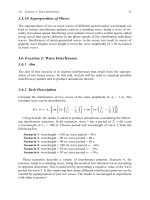
3.6.4 A Glimpse of Results
Figure 3.4 shows a snapshot result for the last scenario. It took me a while to achieve
what I wanted in terms of graphical display and, perhaps, the reader will come up
with a better solution. It can be seen that, at some locations, wave disturbances add
up to create a signal of doubled amplitude, whereas, in other regions, the waves
compensate each other such that the resultant wave signal almost vanishes.
Fig. 3.4 Snapshot results of Scenario 6
3.6.5 A Rule of Thumb
The wave period should be resolved by at least 10 time steps. Otherwise details of
the wave evolution can get lost. In the following SciLab script, I used 20 time steps
in a period. Adequate choices of time steps and grid spacings play an important role
in the modelling of dynamical processes in fluids
3.7 Forces 27
3.7 Forces
3.7.1 What Forces Do
A non-zero force operates to change the speed and/or the direction of motion of a
flui parcel. In geophysical flui dynamics, forces are conventionally expressed as
forces per unit mass, being directly proportional to acceleration or deceleration of
a flui parcel. So, whenever the term “force” appears in the following, this actually
should mean “force per unit mass”.
In component form, a temporal change of the velocity vector can be formally

written as:
du
dt
= F
x
dv
dt
= F
y
dw
dt
= F
z
where (F
x
,F
y
,F
z
) are the vector components of a force of certain magnitude and
direction. For example, (0, 0, −9.81 m/s
2
) is a force operating into the nega-
tive z-direction (downward). With two forces involved, the latter equations can be
written as:
du
dt
= F
x
1

+ F
x
2
dv
dt
= F
y
1
+ F
y
2
dw
dt
= F
z
1
+ F
z
2
Acceleration or deceleration results if any component of the resultant net force is
different from zero. In the general case, the sum symbol “

” can be used to write:
du
dt
=
m

i=1
F

x
i
dv
dt
=
m

i=1
F
y
i
, (3.5)
dw
dt
=
m

i=1
F
z
i
where m is the number of forces involved in a process, and the index i points to a
certain force.
28 3 Basics of Geophysical Fluid Dynamics
3.7.2 Newton’s Laws of Motion
Equations (3.5) already state the firs two of Newton’s laws of motion (Newton,
1687). Newton’s f rst law of motion states that, in an absolute coordinate system
void of any rotation or translation, both speed and direction of motion of a body
remain unchanged in the absence of forces. If there is a force, on the other hand,
there will be a certain change in motion. This is known as Newton’s second law of

motion.
3.7.3 Apparent Forces
Apparent forces come into play in a rotating coordinate system such as our Earth.
One of these apparent forces is the Coriolis force that gives rise to circular weather
patterns in the atmosphere, eddies in the ocean, or Jupiter’s Red Spot.
3.7.4 Lagrangian Trajectories
Imagine that you sit on a flui parcel of a certain temperature moving with the f ow.
The path along which you move is called a Lagrangian trajectory, based on work by
Lagrange (1788). Without any heat exchange with the ambient fluid the temperature
of your flui parcel remains constant and this feature can be formulated as:
dT
dt
= 0 (3.6)
where “T” is temperature and the “d” symbol now refers to a change of temperature
along the pathway of motion.
3.7.5 Eulerian Frame of Reference and Advection
Instead of moving with the f ow, you could stand still at a f xed location and measure
changes in temperatures as the flui moves past. This perspective is called the Eule-
rian system, based on work by Euler (1736). In this case, you would notice a change
in temperature if a fl w exists that carries differences (gradients) in temperature
towards you. This process is called advection. In Cartesian coordinates, the effect
of temperature advection can be expressed as:
∂T
∂t
=−u
∂T
∂x
− v
∂T
∂y

− w
∂T
∂z
(3.7)
This advection equation constitutes a partial differential equation.
3.7 Forces 29
3.7.6 Interpretation of the Advection Equation
The existence of both a f ow and temperature gradients are essential ingredients in
the advection process. The left-hand side of (3.7) is the temporal change in temper-
ature measured at a f xed location. The appearance of minus signs on the right-hand
side of (3.7) is not that difficul to understand. For simplicity, consider a f ow running
parallel to the x-direction. Recall that, per definition u is positive if this fl w com-
ponent runs into the positive x-direction. Warming over time (∂ T /∂t > 0) occurs
with an increase of T in the x-direction in conjunction with a negative u. Warming
also occurs with a positive u but a decrease of T in the x-direction. I am sure that
the reader can work out scenarios leading to a local cooling.
In the absence of either fl w or temperature gradients, Eq. (3.7) turns into:
∂T
∂t
= 0 (3.8)
This equation simply means that temperature does not show changes at a certain
location. The important difference with respect to (3.6) is that this relation holds for
a f xed location, whereas the other one was for an observer moving with the f ow.
Most ocean models use the Eulerian frame of reference.
3.7.7 The Nonlinear Terms
Flow can advect different properties such as gradients in temperature, salinity and
nutrients, but also momentum; that is, the components of velocity itself. The resul-
tant terms are called the nonlinear terms. These terms are included in Newton’s
second law of motion, if we express this in an Eulerian frame of reference, yielding:
∂u

∂t
+ u
∂u
∂x
+ v
∂u
∂y
+ w
∂u
∂z
=
m

i=1
F
x
i
∂v
∂t
+ u
∂v
∂x
+ v
∂v
∂y
+ w
∂v
∂z
=
m


i=1
F
y
i
(3.9)
∂w
∂t
+ u
∂w
∂x
+ v
∂w
∂y
+ w
∂w
∂z
=
m

i=1
F
z
i
The nonlinear terms are traditionally written on the left-hand side of the momen-
tum conservation equations for they are no true forces.
30 3 Basics of Geophysical Fluid Dynamics
3.7.8 Impacts of the Nonlinear Terms
The nonlinear terms are important in the dynamics of many processes. For instance,
these terms are the reason for the existence of turbulence which makes mixing a soup

with a spoon much more efficien than just waiting until the soup has mixed itself.
The reader can also blame these terms for the unreliability of weather forecasts for
longer than 5 days ahead.
3.8 Fundamental Conservation Principles
3.8.1 A List of Principles
There are several conservation principles that need to be considered when studying
flui motions. These are:
1. Conservation of momentum (Newton’s laws of motion)
2. Conservation of mass
3. Conservation of interal energy (heat)
4. Conservation of salt.
In addition to this comes the so-called equation of state that links the fiel vari-
ables such as temperature and salinity to the density of the fluid All these equations
are coupled with each other, which makes the equations describing flui motions a
coupled system of partial differential equations.
3.8.2 Conservation of Momentum
Conservation of momentum is an expression of changes in fl w speed and/or direc-
tion as a result of forces. The frictional stress imposed by winds along the sea surface
acts as a boundary source term in the momentum equations. Friction at the sea f ow
acts as a sink term in these equations. Forces of relevance to fluid are explored in
the next sections.
3.8.3 Conservation of Volume – The Continuity Equation
Water is largely incompressible, so that the mass of a given water volume cannot
change much under compression. Conservation of mass can therefore be expressed
in terms of conservation of volume. To understand this important concept, consider
a virtual volume element (Fig. 3.5). For simplicity, we orientate this element in such
a way that its face normals are parallel to the directions of the Cartesian coordinate
system. The side-lengths of this box are δx, δy and δz, and the volume is δV =
δx · δy · δz.
3.8 Fundamental Conservation Principles 31

Fig. 3.5 A virtual control volume in a Cartesian coordinate system
Flow can enter or escape through any face of this volume element. Incompress-
ibility of a flui implies that all these individual infl ws and outfl ws have to be
balanced. Volume infl w or outfl w is the product of the area of a face of our volume
element and the f ow component normal to it. The eastern and western faces span
an area of δy · δz each and the relative volume change is given by δu · δy · δz, where
δu is the difference of fl w speed between both faces. This relative volume change
can be reformulated as:
δu(δyδz) =
δu
δx
δxδyδz =
δu
δx
δV
Adding the contributions of the three pairs of opposite faces of the volume ele-
ment and requesting this sum to be zero yields:
0 =

δu
δx
+
δv
δy
+
δw
δz

δV
Since δV is a positive and non-zero quantity, the fina equation reads:

δu
δx
+
δv
δy
+
δw
δz
= 0
The equation is valid for any finit volume and, accordingly, for a vanishingly
small volume, which can be expressed by the partial differential equation
∂u
∂x
+
∂v
∂y
+
∂w
∂z
= 0 (3.10)
being called the continuity equation. This equation constitutes the local form of
volume conservation. One shortcoming when assuming an incompressible flui is
that acoustic waves in the flui can no longer be described.