Numerical Methods in Engineering with Python Phần 9 ppt
Bạn đang xem bản rút gọn của tài liệu. Xem và tải ngay bản đầy đủ của tài liệu tại đây (492.65 KB, 44 trang )
P1: PHB
CUUS884-Kiusalaas CUUS884-09 978 0 521 19132 6 December 16, 2009 15:4
341 9.3 Power and Inverse Power Methods
EXAMPLE 9.4
The stress matrix describing the state of stress at a point is
S =
⎡
⎢
⎣
−30 10 20
10 40 −50
20 −50 −10
⎤
⎥
⎦
MPa
Determine the largest principal stress (the eigenvalue of S furthest from zero) by the
power method.
Solution
First iteration:
Let v =
100
T
be the initial guess for the eigenvector. Then,
z = Sv =
⎡
⎢
⎣
−30 10 20
10 40 −50
20 −50 −10
⎤
⎥
⎦
⎡
⎢
⎣
1
0
0
⎤
⎥
⎦
=
⎡
⎢
⎣
−30.0
10.0
20.0
⎤
⎥
⎦
|
z
|
=
30
2
+ 10
2
+ 20
2
= 37.417
v =
z
|
z
|
=
⎡
⎢
⎣
−30.0
10.0
20.0
⎤
⎥
⎦
1
37.417
=
⎡
⎢
⎣
−0.801 77
0.267 26
0.534 52
⎤
⎥
⎦
Second iteration:
z = Sv =
⎡
⎢
⎣
−30 10 20
10 40 −50
20 −50 −10
⎤
⎥
⎦
⎡
⎢
⎣
−0.801 77
0.267 26
0.534 52
⎤
⎥
⎦
=
⎡
⎢
⎣
37.416
−24.053
−34.744
⎤
⎥
⎦
|
z
|
=
37.416
2
+ 24.053
2
+ 34.744
2
= 56. 442
v =
z
|
z
|
=
⎡
⎢
⎣
37.416
−24.053
−34.744
⎤
⎥
⎦
1
56. 442
=
⎡
⎢
⎣
0.66291
−0.42615
−0.61557
⎤
⎥
⎦
Third iteration:
z = Sv =
⎡
⎢
⎣
−30 10 20
10 40 −50
20 −50 −10
⎤
⎥
⎦
⎡
⎢
⎣
0.66291
−0.42615
−0.61557
⎤
⎥
⎦
=
⎡
⎢
⎣
−36.460
20.362
40.721
⎤
⎥
⎦
|
z
|
=
36.460
2
+ 20.362
2
+ 40.721
2
= 58.328
v =
z
|
z
|
=
⎡
⎢
⎣
−36.460
20.362
40.721
⎤
⎥
⎦
1
58.328
=
⎡
⎢
⎣
−0.62509
0.34909
0.69814
⎤
⎥
⎦
P1: PHB
CUUS884-Kiusalaas CUUS884-09 978 0 521 19132 6 December 16, 2009 15:4
342 Symmetric Matrix Eigenvalue Problems
At this point the approximation of the eigenvalue we seek is λ =−58.328 MPa (the
negative sign is determined by the sign reversal of z between iterations). This is actu-
ally close to the second-largest eigenvalue λ
2
=−58.39 MPa. By continuing the itera-
tive process we would eventually end up with the largest eigenvalue λ
3
= 70.94 MPa.
But since
|
λ
2
|
and
|
λ
3
|
are rather close, the convergence is too slow from this point on
for manual labor. Here is a program that does the calculations for us:
#!/usr/bin/python
## example9_4
from numpy import array,dot
from math import sqrt
s = array([[-30.0, 10.0, 20.0], \
[ 10.0, 40.0, -50.0], \
[ 20.0, -50.0, -10.0]])
v = array([1.0, 0.0, 0.0])
for i in range(100):
vOld = v.copy()
z = dot(s,v)
zMag = sqrt(dot(z,z))
v = z/zMag
if dot(vOld,v) < 0.0:
sign = -1.0
v=-v
else: sign = 1.0
if sqrt(dot(vOld - v,vOld - v)) < 1.0e-6: break
lam = sign*zMag
print "Number of iterations =",i
print "Eigenvalue =",lam
raw_input("Press return to exit")
The results are:
Number of iterations = 92
Eigenvalue = 70.9434833068
Note that it took 92 iterations to reach convergence.
EXAMPLE 9.5
Determine the smallest eigenvalue λ
1
and the corresponding eigenvector of
A =
⎡
⎢
⎢
⎢
⎢
⎢
⎣
112314
29352
3315 4 3
15 412 4
42 3 417
⎤
⎥
⎥
⎥
⎥
⎥
⎦
Use the inverse power method with eigenvalue shifting, knowing that λ
1
≈ 5.
P1: PHB
CUUS884-Kiusalaas CUUS884-09 978 0 521 19132 6 December 16, 2009 15:4
343 9.3 Power and Inverse Power Methods
Solution
#!/usr/bin/python
## example9_5
from numpy import array
from inversePower import *
s = 5.0
a = array([[ 11.0, 2.0, 3.0, 1.0, 4.0], \
[ 2.0, 9.0, 3.0, 5.0, 2.0], \
[ 3.0, 3.0, 15.0, 4.0, 3.0], \
[ 1.0, 5.0, 4.0, 12.0, 4.0], \
[ 4.0, 2.0, 3.0, 4.0, 17.0]])
lam,x = inversePower(a,s)
print "Eigenvalue =",lam
print "\nEigenvector:\n",x
raw_input("\nPrint press return to exit")
Here is the output:
Eigenvalue = 4.87394637865
Eigenvector:
[-0.26726603 0.74142854 0.05017271 -0.59491453 0.14970633]
Convergence was achieved with four iterations. Without the eigenvalue shift, 26
iterations would be required.
EXAMPLE 9.6
Unlike Jacobi diagonalization, the inverse power method lends itself to eigenvalue
problems of banded matrices. Write a program that computes the smallest buckling
load of the beam described in Example 9.3, making full use of the banded forms. Run
the program with 100 interior nodes (n = 100).
Solution The function
inversePower5 listed here returns the smallest eigenvalue
and the corresponding eigenvector of Ax = λBx,whereA is a pentadiagonal ma-
trix and B is a sparse matr ix (in this problem it is tridiagonal). The matrix A is in-
put by its diagonals d, e, and f as was done in Section 2.4 in conjunction with the
LU decomposition. The algorithm for
inversePower5 does not use B directly, but
calls the function
Bv(v) that supplies the product Bv. Eigenvalue shifting is not
used.
## module inversePower5
’’’ lam,x = inversePower5(Bv,d,e,f,tol=1.0e-6).
Inverse power method for solving the eigenvalue problem
[A]{x} = lam[B]{x}, where [A] = [f\e\d\e\f] is
pentadiagonal and [B] is sparse User must supply the
P1: PHB
CUUS884-Kiusalaas CUUS884-09 978 0 521 19132 6 December 16, 2009 15:4
344 Symmetric Matrix Eigenvalue Problems
function Bv(v) that returns the vector [B]{v}.
’’’
from numpy import zeros,dot
from LUdecomp5 import *
from math import sqrt
from random import random
def inversePower5(Bv,d,e,f,tol=1.0e-6):
n = len(d)
d,e,f = LUdecomp5(d,e,f)
x = zeros(n)
for i in range(n): # Seed {v} with random numbers
x[i] = random()
xMag = sqrt(dot(x,x)) # Normalize {v}
x = x/xMag
for i in range(30): # Begin iterations
xOld = x.copy() # Save current {v}
x = Bv(xOld) # Compute [B]{v}
x = LUsolve5(d,e,f,x) # Solve [A]{z} = [B]{v}
xMag = sqrt(dot(x,x)) # Normalize {z}
x = x/xMag
if dot(xOld,x) < 0.0: # Detect change in sign of {x}
sign = -1.0
x=-x
else: sign = 1.0
if sqrt(dot(xOld - x,xOld - x)) < tol:
return sign/xMag,x
print ’Inverse power method did not converge’
The program that utilizes inversePower5 is
#!/usr/bin/python
## example9_6
from numpy import ones,zeros
from inversePower5 import *
def Bv(v): # Compute {z} = [B]{v}
n = len(v)
z = zeros(n)
z[0] = 2.0*v[0] - v[1]
for i in range(1,n-1):
z[i] = -v[i-1] + 2.0*v[i] - v[i+1]
z[n-1] = -v[n-2] + 2.0*v[n-1]
return z
P1: PHB
CUUS884-Kiusalaas CUUS884-09 978 0 521 19132 6 December 16, 2009 15:4
345 9.3 Power and Inverse Power Methods
n = 100 # Number of interior nodes
d = ones(n*6.0 # Specify diagonals of [A] = [f\e\d\e\f]
d[0] = 5.0
d[n-1] = 7.0
e = ones(n-1)*(-4.0)
f = ones(n-2)*1.0
lam,x = inversePower5(Bv,d,e,f)
print "PLˆ2/EI =",lam*(n+1)**2
raw_input("\nPress return to exit")
The output is in excellent agreement with the analytical value:
PLˆ2/EI = 20.1867355603
PROBLEM SET 9.1
1. Given
A =
⎡
⎢
⎣
731
396
168
⎤
⎥
⎦
B =
⎡
⎢
⎣
400
090
004
⎤
⎥
⎦
convert the eigenvalue problem Ax = λBx to the standard form Hz = λz.Whatis
the relationship between x and z?
2. Convert the eigenvalue problem Ax = λBx,where
A =
⎡
⎢
⎣
4 −10
−14−1
0 −14
⎤
⎥
⎦
B =
⎡
⎢
⎣
2 −10
−12−1
0 −11
⎤
⎥
⎦
to the standard form.
3. An eigenvalue of the problem in Prob. 2 is roughly 2.5. Use the inverse power
method with eigenvalue shifting to compute this eigenvalue to four decimal
places. Start with x =
100
T
. Hint: two iterations should be sufficient.
4. The stress matrix at a point is
S =
⎡
⎢
⎣
150 −60 0
−60 120 0
0080
⎤
⎥
⎦
MPa
Compute the principal stresses (eigenvalues of S).
5.
m
m
LL
k
θ
θ
1
2
2
P1: PHB
CUUS884-Kiusalaas CUUS884-09 978 0 521 19132 6 December 16, 2009 15:4
346 Symmetric Matrix Eigenvalue Problems
The two pendulums are connected by a spring that is undeformed when the pen-
dulums are vertical. The equations of motion of the system can be shown to be
kL(θ
2
− θ
1
) −mgθ
1
= mL
¨
θ
1
−kL(θ
2
− θ
1
) −2mgθ
2
= 2mL
¨
θ
2
where θ
1
and θ
2
are the angular displacements and k is the spring stiffness.
Determine the circular frequencies of vibration and the relative amplitudes of
the angular displacements. Use m = 0.25 kg, k = 20 N/m, L = 0.75 m, and g =
9.80665 m/s
2
.
6.
L
L
L
C
C
C
i
1
i
2
i
3
i
1
i
2
i
3
Kirchoff’s laws for the electric circuit are
3i
1
−i
2
−i
3
=−LC
d
2
i
1
dt
2
−i
1
+i
2
=−LC
d
2
i
2
dt
2
−i
1
+i
3
=−LC
d
2
i
3
dt
2
Compute the circular frequencies of the circuit and the relative amplitudes of the
loop currents.
7. Compute the matrix A
∗
that results from annihilation A
14
and A
41
in the matrix
A =
⎡
⎢
⎢
⎢
⎣
4 −101
−16−20
0 −232
1024
⎤
⎥
⎥
⎥
⎦
by a Jacobi rotation.
8.
Use the Jacobi method to determine the eigenvalues and eigenvectors of
A =
⎡
⎢
⎣
4 −12
−133
−231
⎤
⎥
⎦
P1: PHB
CUUS884-Kiusalaas CUUS884-09 978 0 521 19132 6 December 16, 2009 15:4
347 9.3 Power and Inverse Power Methods
9. Find the eigenvalues and eigenvectors of
A =
⎡
⎢
⎢
⎢
⎣
4 −21−1
−24−21
1 −24−2
−11−24
⎤
⎥
⎥
⎥
⎦
with the Jacobi method.
10.
Use the power method to compute the largest eigenvalue and the correspond-
ing eigenvector of the matrix A given in Prob. 9.
11.
Find the smallest eigenvalue and the corresponding eigenvector of the matrix
A in Prob. 9. Use the inverse power method.
12.
Let
A =
⎡
⎢
⎣
1.40.80.4
0.86.60.8
0.40.85.0
⎤
⎥
⎦
B =
⎡
⎢
⎣
0.4 −0.10.0
−0.10.4 −0.1
0.0 −0.10.4
⎤
⎥
⎦
Find the eigenvalues and eigenvectors of Ax = λBx by the Jacobi method.
13.
Use the inverse power method to compute the smallest eigenvalue in Prob. 12.
14.
Use the Jacobi method to compute the eigenvalues and eigenvectors of the
matrix
A =
⎡
⎢
⎢
⎢
⎢
⎢
⎢
⎢
⎢
⎣
1123142
29 3 5 21
3315 4 32
15 412 43
42 3 4175
21 2 3 58
⎤
⎥
⎥
⎥
⎥
⎥
⎥
⎥
⎥
⎦
15.
Find the eigenvalues of Ax = λBx by the Jacobi method, where
A =
⎡
⎢
⎢
⎢
⎣
6 −410
−46−41
1 −46−4
01−47
⎤
⎥
⎥
⎥
⎦
B =
⎡
⎢
⎢
⎢
⎣
1 −23−1
−26−23
3 −26−2
−13−29
⎤
⎥
⎥
⎥
⎦
Warning : B is not positive definite.
16.
1
n
2
L
x
u
The figure shows a cantilever beam with a superimposed finite difference mesh.
If u(x, t) is the lateral displacement of the beam, the differential equation of mo-
tion governing bending vibrations is
u
(4)
=−
γ
EI
¨
u
P1: PHB
CUUS884-Kiusalaas CUUS884-09 978 0 521 19132 6 December 16, 2009 15:4
348 Symmetric Matrix Eigenvalue Problems
where γ is the mass per unit length and EI is the bending rigidity. The bound-
ary conditions are u(0, t) = u
(0, t) = u
(L, t) = u
(L, t) = 0. With u(x, t) = y(x)
sin ωt the problem becomes
y
(4)
=
ω
2
γ
EI
yy(0) = y
(0) = y
(L) = y
(L) = 0
The corresponding finite difference equations are
A =
⎡
⎢
⎢
⎢
⎢
⎢
⎢
⎢
⎢
⎢
⎢
⎢
⎣
7 −4100··· 0
−46−410··· 0
1 −46−41··· 0
.
.
.
.
.
.
.
.
.
.
.
.
.
.
.
.
.
.
.
.
.
0 ··· 1 −46−41
0 ··· 01−45−2
0 ··· 001−21
⎤
⎥
⎥
⎥
⎥
⎥
⎥
⎥
⎥
⎥
⎥
⎥
⎦
⎡
⎢
⎢
⎢
⎢
⎢
⎢
⎢
⎢
⎢
⎢
⎢
⎣
y
1
y
2
y
3
.
.
.
y
n−2
y
n−1
y
n
⎤
⎥
⎥
⎥
⎥
⎥
⎥
⎥
⎥
⎥
⎥
⎥
⎦
= λ
⎡
⎢
⎢
⎢
⎢
⎢
⎢
⎢
⎢
⎢
⎢
⎢
⎣
y
1
y
2
y
3
.
.
.
y
n−2
y
n−1
y
n
/2
⎤
⎥
⎥
⎥
⎥
⎥
⎥
⎥
⎥
⎥
⎥
⎥
⎦
where
λ =
ω
2
γ
EI
L
n
4
(a) Write down the matrix H of the standard form Hz = λz and the transforma-
tion matrix P as in y = Pz. (b) Write a program that computes the lowest two
circular frequencies of the beam and the corresponding mode shapes (eigenvec-
tors) using the Jacobi method. Run the program with n = 10. Note: the analytical
solution for the lowest circular frequency is ω
1
=
3.515/L
2
√
EI/γ .
17.
120 345678910
L
L
/4
/4
(b)
P
P
L
LL
EI
EI
2
/2
/4
/4
0
0
EI
0
(a)
The simply supported column in Fig. (a) consists of three segments with the
bending rigidities shown. If only the first buckling mode is of interest, it is suf-
ficient to model half of the beam as shown in Fig. (b). The differential equation
for the lateral displacement u(x)is
u
=−
P
EI
u
P1: PHB
CUUS884-Kiusalaas CUUS884-09 978 0 521 19132 6 December 16, 2009 15:4
349 9.3 Power and Inverse Power Methods
with the boundary conditions u(0) = u
(0) = 0. The corresponding finite differ-
ence equations are
⎡
⎢
⎢
⎢
⎢
⎢
⎢
⎢
⎢
⎢
⎢
⎢
⎢
⎢
⎢
⎢
⎢
⎣
2 −100000··· 0
−12−10000··· 0
0 −12−1000··· 0
00−12−100··· 0
000−12−10··· 0
0000−12−1 ··· 0
.
.
.
.
.
.
.
.
.
.
.
.
.
.
.
.
.
.
.
.
.
.
.
.
.
.
.
0 ··· 0000−12−1
0 ··· 00000−11
⎤
⎥
⎥
⎥
⎥
⎥
⎥
⎥
⎥
⎥
⎥
⎥
⎥
⎥
⎥
⎥
⎥
⎦
⎡
⎢
⎢
⎢
⎢
⎢
⎢
⎢
⎢
⎢
⎢
⎢
⎢
⎢
⎢
⎢
⎢
⎣
u
1
u
2
u
3
u
4
u
5
u
6
.
.
.
u
9
u
10
⎤
⎥
⎥
⎥
⎥
⎥
⎥
⎥
⎥
⎥
⎥
⎥
⎥
⎥
⎥
⎥
⎥
⎦
= λ
⎡
⎢
⎢
⎢
⎢
⎢
⎢
⎢
⎢
⎢
⎢
⎢
⎢
⎢
⎢
⎢
⎢
⎣
u
1
u
2
u
3
u
4
u
5
/1.5
u
6
/2
.
.
.
u
9
/2
u
10
/4
⎤
⎥
⎥
⎥
⎥
⎥
⎥
⎥
⎥
⎥
⎥
⎥
⎥
⎥
⎥
⎥
⎥
⎦
where
λ =
P
EI
0
L
20
2
Write a program that computes the lowest buckling load P of the column with
the inverse power method. Utilize the banded forms of the matrices.
18.
θ
3
θ
2
θ
1
L
L
L
k
k
k
P
The springs supporting the three-bar linkage are undeformed when the linkage
is horizontal. The equilibrium equations of the linkage in the presence of the
horizontal force P can be shown to be
⎡
⎢
⎣
653
332
111
⎤
⎥
⎦
⎡
⎢
⎣
θ
1
θ
2
θ
3
⎤
⎥
⎦
=
P
kL
⎡
⎢
⎣
111
011
001
⎤
⎥
⎦
⎡
⎢
⎣
θ
1
θ
2
θ
3
⎤
⎥
⎦
where k is the spring stiffness. Determine the smallest buckling load P and the
corresponding mode shape. Hint: The equations can easily rewritten in the stan-
dard form Aθ = λθ,whereA is symmetric.
19.
m
2
m
3
m
k
k
kk
u
u
u
1
2
3
The differential equations of motion for the mass-spring system are
k
(
−2u
1
+u
2
)
= m
¨
u
1
k(u
1
− 2u
2
+u
3
) = 3m
¨
u
2
k(u
2
− 2u
3
) = 2m
¨
u
3
P1: PHB
CUUS884-Kiusalaas CUUS884-09 978 0 521 19132 6 December 16, 2009 15:4
350 Symmetric Matrix Eigenvalue Problems
where u
i
(t) is the displacement of mass i from its equilibrium position and k is
the spring stiffness. Determine the circular frequencies of vibration and the cor-
responding mode shapes.
20.
L
L
L
L
C
C
/5
C/2
C
/3
C/4
i
1
i
2
i
3
i
4
i
1
i
2
i
3
i
4
Kirchoff’s equations for the circuit are
L
d
2
i
1
dt
2
+
1
C
i
1
+
2
C
(i
1
−i
2
) = 0
L
d
2
i
2
dt
2
+
2
C
(i
2
−i
1
) +
3
C
(i
2
−i
3
) = 0
L
d
2
i
3
dt
2
+
3
C
(i
3
−i
2
) +
4
C
(i
3
−i
4
) = 0
L
d
2
i
4
dt
2
+
4
C
(i
4
−i
3
) +
5
C
i
4
= 0
Find the circular frequencies of the current.
21.
L
LL
L
C
C
/2
C
/3
C/4
i
1
i
2
i
3
i
4
i
1
i
2
i
3
i
4
L
Determine the circular frequencies of oscillation for the circuit shown, given the
Kirchoff equations
L
d
2
i
1
dt
2
+ L
d
2
i
1
dt
2
−
d
2
i
2
dt
2
+
1
C
i
1
= 0
L
d
2
i
2
dt
2
−
d
2
i
1
dt
2
+ L
d
2
i
2
dt
2
−
d
2
i
3
dt
2
+
2
C
= 0
L
d
2
i
3
dt
2
−
d
2
i
2
dt
2
+ L
d
2
i
3
dt
2
−
d
2
i
4
dt
2
+
3
C
i
3
= 0
L
d
2
i
4
dt
2
−
d
2
i
3
dt
2
+ L
d
2
i
4
dt
2
+
4
C
i
4
= 0
22.
Several iterative methods exist for finding the eigenvalues of a matrix A.Oneof
these is the LR method, which requires the matrix to be symmetric and positive
P1: PHB
CUUS884-Kiusalaas CUUS884-09 978 0 521 19132 6 December 16, 2009 15:4
351 9.4 Householder Reduction to Tridiagonal Form
definite. Its algorithm is very simple:
Let A
0
= A
do withi = 0, 1, 2,
Use Choleski’s decomposition A
i
= L
i
L
T
i
to compute L
i
Form A
i+1
= L
T
i
L
i
end do
It can be shown that the diagonal elements of A
i+1
converge to the eigenvalues
of A. Write a program that implements the LR method and test it with
A =
⎡
⎢
⎣
431
342
123
⎤
⎥
⎦
9.4 Householder Reduction to Tridiagonal Form
It was mentioned before that similarity transformations can be used to transform an
eigenvalue problem to a form that is easier to solve. The most desirable of the “easy”
forms is, of course, the diagonal for m that results from the Jacobi method. However,
the Jacobi method requires about 10n
3
to 20n
3
multiplications, so that the amount of
computation increases very rapidly with n. We are generally better off by reducing the
matrix to the tridiagonal form, which can be done in precisely n −2 transformations
by the Householder method. Once the tridiagonal form is achieved, we still have to
extract the eigenvalues and the eigenvectors, but there are effective means of dealing
with that, as we see in the next section.
Householder Matrix
Each Householder transformation utilizes the Householder matrix
Q = I −
uu
T
H
(9.36)
where u is a vector and
H =
1
2
u
T
u =
1
2
|
u
|
2
(9.37)
Note that uu
T
in Eq. (9.36) is the outer product, that is, a matrix with the elements
uu
T
ij
= u
i
u
j
. Because Q is obviously symmetric (Q
T
= Q), we can write
Q
T
Q = QQ =
I −
uu
T
H
I −
uu
T
H
= I −2
uu
T
H
+
u
u
T
u
u
T
H
2
= I − 2
uu
T
H
+
u
(
2H
)
u
T
H
2
= I
which shows that Q is also orthogonal.
P1: PHB
CUUS884-Kiusalaas CUUS884-09 978 0 521 19132 6 December 16, 2009 15:4
352 Symmetric Matrix Eigenvalue Problems
Now let x be an arbitrary vector and consider the transformation Qx. Choosing
u = x + ke
1
(9.38)
where
k =±
|
x
|
e
1
=
100··· 0
T
we g et
Qx =
I −
uu
T
H
x =
I −
u
x +ke
1
T
H
x
= x −
u
x
T
x+ke
T
1
x
H
= x −
u
k
2
+ kx
1
H
But
2H =
x +ke
1
T
x +ke
1
=
|
x
|
2
+ k
x
T
e
1
+e
T
1
x
+ k
2
e
T
1
e
1
= k
2
+ 2kx
1
+ k
2
= 2
k
2
+ kx
1
so that
Qx = x − u =−ke
1
=
−k 00··· 0
T
(9.39)
Hence, the transformation eliminates all elements of x except the first one.
Householder Reduction of a Symmetric Matrix
Let us now apply the following transformation to a symmetric n ×n matrix A:
P
1
A =
1 0
T
0Q
A
11
x
T
xA
=
A
11
x
T
Qx QA
(9.40)
Here x represents the first column of A with the first element omitted, and A
is sim-
ply A with its first row and column removed. The matrix Q of dimensions (n −1) ×
(n − 1) is constructed using Eqs. (9.36)–(9.38). Referring to Eq. (9.39), we see that the
transformation reduces the first column of A to
A
11
Qx
=
⎡
⎢
⎢
⎢
⎢
⎢
⎢
⎣
A
11
−k
0
.
.
.
0
⎤
⎥
⎥
⎥
⎥
⎥
⎥
⎦
The transformation
A ← P
1
AP
1
=
A
11
Qx
T
Qx QA
Q
(9.41)
P1: PHB
CUUS884-Kiusalaas CUUS884-09 978 0 521 19132 6 December 16, 2009 15:4
353 9.4 Householder Reduction to Tridiagonal Form
thus tridiagonalizes the first row as well as the first column of A.Hereisadiagramof
the transformation for a 4 × 4matrix:
1 00 0
0
0 Q
0
·
A
11
A
12
A
13
A
14
A
21
A
31
A
A
41
·
1 00 0
0
0 Q
0
=
A
11
−k 00
−k
0 QA
Q
0
The second row and column of A are reduced next by applying the transformation to
the 3 ×3 lower right portion of the matrix. This transformation can be expressed as
A ← P
2
AP
2
, where now
P
2
=
I
2
0
T
0Q
(9.42)
In Eq. (9.42), I
2
is a 2 ×2 identity matr ix and Q is a (n − 2) × (n −2) matrix con-
structed by choosing for x the bottom n −2 elements of the second column of A.
It takes a total of n − 2 transformations with
P
i
=
I
i
0
T
0Q
, i = 1, 2, , n − 2
to attain the tridiagonal form.
It is wasteful to form P
i
and to carry out the matrix multiplication P
i
AP
i
. We note
that
A
Q = A
I −
uu
T
H
= A
−
A
u
H
u
T
= A
−vu
T
where
v =
A
u
H
(9.43)
Therefore,
QA
Q =
I −
uu
T
H
A
−vu
T
= A
−vu
T
−
uu
T
H
A
−vu
T
= A
−vu
T
−
u
u
T
A
H
+
u
u
T
v
u
T
H
= A
−vu
T
−uv
T
+ 2guu
T
where
g =
u
T
v
2H
(9.44)
P1: PHB
CUUS884-Kiusalaas CUUS884-09 978 0 521 19132 6 December 16, 2009 15:4
354 Symmetric Matrix Eigenvalue Problems
Letting
w = v − gu (9.45)
it can be easily verified that the transformation can be written as
QA
Q = A
−wu
T
−uw
T
(9.46)
which gives us the following computational procedure that is to be carried out with
i = 1, 2, , n − 2:
1. Let A
be the (n −i) ×
n −i
lower right-hand portion of A.
2. Let x =
A
i+1,i
A
i+2,i
··· A
n,i
T
(the column of length n −i just left of A
).
3. Compute
|
x
|
.Letk =
|
x
|
if x
1
> 0 and k =−
|
x
|
if x
1
< 0 (this choice of sign mini-
mizes the roundoff error).
4. Let u =
k+x
1
x
2
x
3
··· x
n−i
T
.
5. Compute H =
|
u
|
/2.
6. Compute v = A
u/H.
7. Compute g = u
T
v/(2H).
8. Compute w = v −gu.
9. Compute the transformation A
← A
−w
T
u −u
T
w.
10. Set A
i,i+1
= A
i+1,i
=−k.
Accumulated Transformation Matrix
Because we used similarity transformations, the eigenvalues of the tridiagonal matrix
are the same as those of the original matrix. However, to determine the eigenvectors
X of original A, we must use the transformation
X = PX
tridiag
where P is the accumulation of the individual transformations:
P = P
1
P
2
···P
n−2
We build up the accumulated transformation matrix by initializing P to an n ×n iden-
tity matrix and then applying the transformation
P ← PP
i
=
P
11
P
12
P
21
P
22
I
i
0
T
0Q
=
P
11
P
21
Q
P
12
P
22
Q
(b)
with i = 1, 2, , n −2. It can be seen that each multiplication affects only the right-
most n −i columns of P (because the first row of P
12
contains only zeroes, it can also
be omitted in the multiplication). Using the notation
P
=
P
12
P
22
P1: PHB
CUUS884-Kiusalaas CUUS884-09 978 0 521 19132 6 December 16, 2009 15:4
355 9.4 Householder Reduction to Tridiagonal Form
we h ave
P
12
Q
P
22
Q
= P
Q = P
I −
uu
T
H
= P
−
P
u
H
u
T
= P
−yu
T
(9.47)
where
y =
P
u
H
(9.48)
The procedure for carrying out the matrix multiplication in Eq. (b) is:
• Retrieve u (in our triangularization procedure the u’s are stored in the columns
of the lower triangular portion of A).
• Compute H =
|
u
|
/2.
• Compute y = P
u/H.
• Compute the transformation P
← P
−yu
T
.
householder
The function householder in this module does the triangulization. It returns (d, c),
where d and c are vectors that contain the elements of the principal diagonal and the
subdiagonal, respectively. Only the upper triangular portion is reduced to the trian-
gular form. The part below the principal diagonal is used to store the vectors u.Thisis
done automatically by the statement
u = a[k+1:n,k], which does not create a new
object
u, but simply sets up a reference to a[k+1:n,k] (makes a deep copy). Thus,
any changes made to
u are reflected in a[k+1:n,k].
The function
computeP returns the accumulated transformation matrix P.There
is no need to call it if only the eigenvalues are to be computed.
## module householder
’’’ d,c = householder(a).
Householder similarity transformation of matrix [a] to
the tridiagonal form [c\d\c].
p = computeP(a).
Computes the acccumulated transformation matrix [p]
after calling householder(a).
’’’
from numpy import dot,diagonal,outer,identity
from math import sqrt
def householder(a):
n = len(a)
for k in range(n-2):
u = a[k+1:n,k]
uMag = sqrt(dot(u,u))
if u[0] < 0.0: uMag = -uMag
P1: PHB
CUUS884-Kiusalaas CUUS884-09 978 0 521 19132 6 December 16, 2009 15:4
356 Symmetric Matrix Eigenvalue Problems
u[0] = u[0] + uMag
h = dot(u,u)/2.0
v = dot(a[k+1:n,k+1:n],u)/h
g = dot(u,v)/(2.0*h)
v=v-g*u
a[k+1:n,k+1:n] = a[k+1:n,k+1:n] - outer(v,u) \
- outer(u,v)
a[k,k+1] = -uMag
return diagonal(a),diagonal(a,1)
def computeP(a):
n = len(a)
p = identity(n)*1.0
for k in range(n-2):
u = a[k+1:n,k]
h = dot(u,u)/2.0
v = dot(p[1:n,k+1:n],u)/h
p[1:n,k+1:n] = p[1:n,k+1:n] - outer(v,u)
return p
EXAMPLE 9.7
Transform the matrix
A =
⎡
⎢
⎢
⎢
⎣
72 3−1
28 5 1
3512 9
−11 9 7
⎤
⎥
⎥
⎥
⎦
into tridiagonal form.
Solution Reduce the first row and column:
A
=
⎡
⎢
⎣
851
5129
197
⎤
⎥
⎦
x =
⎡
⎢
⎣
2
3
−1
⎤
⎥
⎦
k =
|
x
|
= 3. 7417
u =
⎡
⎢
⎣
k + x
1
x
2
x
3
⎤
⎥
⎦
=
⎡
⎢
⎣
5.7417
3
−1
⎤
⎥
⎦
H =
1
2
|
u
|
2
= 21. 484
uu
T
=
⎡
⎢
⎣
32.967 17 225 −5.7417
17.225 9 −3
−5.7417 −31
⎤
⎥
⎦
Q = I−
uu
T
H
=
⎡
⎢
⎣
−0.53450 −0.80176 0.26725
−0.80176 0.58108 0.13964
0.26725 0.13964 0.95345
⎤
⎥
⎦
P1: PHB
CUUS884-Kiusalaas CUUS884-09 978 0 521 19132 6 December 16, 2009 15:4
357 9.4 Householder Reduction to Tridiagonal Form
QA
Q =
⎡
⎢
⎣
10.642 −0.1388 −9.1294
−0.1388 5.9087 4.8429
−9.1294 4.8429 10.4480
⎤
⎥
⎦
A ←
A
11
Qx
T
Qx QA
Q
=
⎡
⎢
⎢
⎢
⎣
7 −3.7417 0 0
−3.7417 10.642 −0. 1388 −9.1294
0 −0.1388 5.9087 4.8429
0 −9.1294 4.8429 10.4480
⎤
⎥
⎥
⎥
⎦
In the last step, we used the formula Qx =
−k 0 ··· 0
T
.
Reduce the second row and column:
A
=
5.9087 4.8429
4.8429 10.4480
x =
−0.1388
−9.1294
k =−
|
x
|
=−9.1305
where the negative sign of k was determined by the sign of x
1
.
u =
k + x
1
−9.1294
=
−9. 2693
−9.1294
H =
1
2
|
u
|
2
= 84.633
uu
T
=
85.920 84.623
84.623 83.346
Q = I−
uu
T
H
=
0.01521 −0.99988
−0.99988 0.01521
QA
Q =
10.594 4.772
4.772 5.762
A ←
⎡
⎢
⎣
A
11
A
12
0
T
A
21
A
22
Qx
T
0QxQA
Q
⎤
⎥
⎦
⎡
⎢
⎢
⎢
⎣
7 −3.742 0 0
−3.742 10.642 9.131 0
09.131 10.594 4.772
0 −04.772 5.762
⎤
⎥
⎥
⎥
⎦
EXAMPLE 9.8
Use the function
householder to tridiagonalize the matrix in Example 9.7; also de-
termine the transformation matrix P.
Solution
#!/usr/bin/python
## example9_8
from numpy import array
from householder import *
P1: PHB
CUUS884-Kiusalaas CUUS884-09 978 0 521 19132 6 December 16, 2009 15:4
358 Symmetric Matrix Eigenvalue Problems
a = array([[ 7.0, 2.0, 3.0, -1.0], \
[ 2.0, 8.0, 5.0, 1.0], \
[ 3.0, 5.0, 12.0, 9.0], \
[-1.0, 1.0, 9.0, 7.0]])
d,c = householder(a)
print "Principal diagonal {d}:\n", d
print "\nSubdiagonal {c}:\n",c
print "\nTransformation matrix [P]:"
print computeP(a)
raw_input("\nPress return to exit")
The results of running the foregoing program are:
Principal diagonal {d}:
[ 7. 10.64285714 10.59421525 5.76292761]
Subdiagonal {c}:
[-3.74165739 9.13085149 4.77158058]
Transformation matrix [P]:
[[ 1. 0. 0. 0. ]
[ 0. -0.53452248 -0.25506831 0.80574554]
[ 0. -0.80178373 -0.14844139 -0.57888514]
[ 0. 0.26726124 -0.95546079 -0.12516436]]
9.5 Eigenvalues of Symmetric Tridiagonal Matrices
Sturm Sequence
In principle, the eigenvalues of a matrix A can be determined by finding the roots of
the characteristic equation
|
A −λI
|
= 0. This method is impractical for large matri-
ces, because the evaluation of the deter minant involves n
3
/3 multiplications. How-
ever, if the matrix is tridiagonal (we also assume it to be symmetric), its characteristic
polynomial
P
n
(λ) =
|
A−λI
|
=
d
1
− λ c
1
00··· 0
c
1
d
2
− λ c
2
0 ··· 0
0 c
2
d
3
− λ c
3
··· 0
00c
3
d
4
− λ ··· 0
.
.
.
.
.
.
.
.
.
.
.
.
.
.
.
.
.
.
00 0 c
n−1
d
n
− λ
P1: PHB
CUUS884-Kiusalaas CUUS884-09 978 0 521 19132 6 December 16, 2009 15:4
359 9.5 Eigenvalues of Symmetric Tridiagonal Matrices
can be computed with only 3(n −1) multiplications using the following sequence of
operations:
P
0
(λ) = 1
P
1
(λ) = d
1
− λ (9.49)
P
i
(λ) = (d
i
− λ)P
i−1
(λ) −c
2
i−1
P
i−2
(λ), i = 2, 3, , n
The polynomials P
0
(λ), P
1
(λ), , P
n
(λ)formaSturm sequence that has the fol-
lowing property:
• The number of sign changes in the sequence P
0
(a), P
1
(a), , P
n
(a)isequalto
the number of roots of P
n
(λ) that are smaller than a. If a member P
i
(a)ofthe
sequence is zero, its sign is to be taken opposite to that of P
i−1
(a).
As we see later, the Sturm sequence property makes it possible to bracket the
eigenvalues of a tridiagonal matrix.
sturmSeq
Given d, c, and λ, the function sturmSeq returns the Sturm sequence
P
0
(λ), P
1
(λ), P
n
(λ)
The function
numLambdas returns the number of sign changes in the sequence (as
noted before, this equals the number of eigenvalues that are smaller than λ).
## module sturmSeq
’’’ p = sturmSeq(c,d,lam).
Returns the Sturm sequence {p[0],p[1], ,p[n]}
associated with the characteristic polynomial
|[A] - lam[I]| = 0, where [A] = [c\d\c] is a n x n
tridiagonal matrix.
numLam = numLambdas(p).
Returns the number of eigenvalues of a tridiagonal
matrix [A] = [c\d\c] that are smaller than ’lam’.
Uses the Sturm sequence {p} obtained from ’sturmSeq’.
’’’
from numpy import ones
def sturmSeq(d,c,lam):
n = len(d) + 1
p = ones(n)
p[1] = d[0] - lam
for i in range(2,n):
P1: PHB
CUUS884-Kiusalaas CUUS884-09 978 0 521 19132 6 December 16, 2009 15:4
360 Symmetric Matrix Eigenvalue Problems
## if c[i-2] == 0.0: c[i-2] = 1.0e-12
p[i] = (d[i-1] - lam)*p[i-1] - (c[i-2]**2)*p[i-2]
return p
def numLambdas(p):
n = len(p)
signOld = 1
numLam = 0
for i in range(1,n):
if p[i] > 0.0: sign = 1
elif p[i] < 0.0: sign = -1
else: sign = -signOld
if sign*signOld < 0: numLam = numLam + 1
signOld = sign
return numLam
EXAMPLE 9.9
Use the Sturm sequence property to show that the smallest eigenvalue of A is in the
interval (0.25, 0.5), where
A =
⎡
⎢
⎢
⎢
⎣
2 −100
−12−10
0 −12−1
00−12
⎤
⎥
⎥
⎥
⎦
Solution Taking λ = 0.5, we have d
i
− λ = 1.5 and c
2
i−1
= 1 and the Sturm sequence
in Eqs. (9.49) becomes
P
0
(0.5) = 1
P
1
(0.5) = 1.5
P
2
(0.5) = 1.5(1.5) − 1 = 1.25
P
3
(0.5) = 1.5(1.25) − 1.5 = 0.375
P
4
(0.5) = 1.5(0.375) − 1.25 =−0.6875
Because the sequence contains one sign change, there exists one eigenvalue smaller
than 0.5.
Repeating the process with λ = 0.25, we get d
i
− λ = 1.75 and c
2
i
= 1, which re-
sults in the Sturm sequence
P
0
(0.25) = 1
P
1
(0.25) = 1.75
P
2
(0.25) = 1.75(1.75) − 1 = 2.0625
P
3
(0.25) = 1.75(2.0625) − 1.75 = 1.8594
P
4
(0.25) = 1.75(1.8594) − 2.0625 = 1.1915
P1: PHB
CUUS884-Kiusalaas CUUS884-09 978 0 521 19132 6 December 16, 2009 15:4
361 9.5 Eigenvalues of Symmetric Tridiagonal Matrices
There are no sign changes in the sequence, so that all the eigenvalues are greater than
0.25. We thus conclude that 0.25 <λ
1
< 0.5.
Gerschgorin’s Theorem
Gerschgorin’s theorem is useful in determining the global bounds on the eigenval-
uesofann ×n matrix A. The term “global” means the bounds that enclose all the
eigenvalues. Here we give a simplified version for a symmetric matrix.
• If λ is an eigenvalue of A,then
a
i
−r
i
≤ λ ≤ a
i
+r
i
, i = 1, 2, , n
where
a
i
= A
ii
r
i
=
n
j =1
j =i
A
ij
(9.50)
It follows that the limits on the smallest and the largest eigenvalues are given by
λ
min
≥ min
i
(a
i
−r
i
) λ
max
≤ max
i
(a
i
+r
i
) (9.51)
gerschgorin
The function gerschgorin returns the lower and upper global bounds on the eigen-
values of a symmetric tridiagonal matrix A = [c\d\c].
## module gerschgorin
’’’ lamMin,lamMax = gerschgorin(d,c).
Applies Gerschgorin’s theorem to find the global bounds on
the eigenvalues of a tridiagomal matrix [A] = [c\d\c].
’’’
def gerschgorin(d,c):
n = len(d)
lamMin = d[0] - abs(c[0])
lamMax = d[0] + abs(c[0])
for i in range(1,n-1):
lam = d[i] - abs(c[i]) - abs(c[i-1])
if lam < lamMin: lamMin = lam
lam = d[i] + abs(c[i]) + abs(c[i-1])
if lam > lamMax: lamMax = lam
lam = d[n-1] - abs(c[n-2])
if lam < lamMin: lamMin = lam
lam = d[n-1] + abs(c[n-2])
if lam > lamMax: lamMax = lam
return lamMin,lamMax
P1: PHB
CUUS884-Kiusalaas CUUS884-09 978 0 521 19132 6 December 16, 2009 15:4
362 Symmetric Matrix Eigenvalue Problems
EXAMPLE 9.10
Use Gerschgorin’s theorem to determine the bounds on the eigenvalues of the matrix
A =
⎡
⎢
⎣
4 −20
−24−2
0 −25
⎤
⎥
⎦
Solution Referring to Eqs. (9.50), we get
a
1
= 4 a
2
= 4 a
3
= 5
r
1
= 2 r
2
= 4 r
3
= 2
Hence,
λ
min
≥ min(a
i
−r
i
) = 4 − 4 = 0
λ
max
≤ max(a
i
+r
i
) = 4 + 4 = 8
Bracketing Eigenvalues
The Sturm sequence property together with Gerschgorin’s theorem provide us con-
venient tools for bracketing each eigenvalue of a symmetric tridiagonal matrix.
lamRange
The function lamRange brackets the N smallest eigenvalues of a symmetric tridi-
agonal matrix A = [c\d\c]. It returns the sequence r
0
, r
1
, , r
N
, where each interval
r
i−1
, r
i
contains exactly one eigenvalue. The algorithm first finds the bounds on all
the eigenvalues by Gerschgorin’s theorem. Then the method of bisection in conjunc-
tion with Sturm sequence property is used to determine r
N
, r
N−1
, , r
0
in that order.
## module lamRange
’’’ r = lamRange(d,c,N).
Returns the sequence {r[0],r[1], ,r[N]} that
separates the N lowest eigenvalues of the tridiagonal
matrix [A] = [c\d\c]; that is, r[i] < lam[i] < r[i+1].
’’’
from numpy import ones
from sturmSeq import *
from gerschgorin import *
def lamRange(d,c,N):
lamMin,lamMax = gerschgorin(d,c)
r = ones(N+1)
r[0] = lamMin
# Search for eigenvalues in descending order
for k in range(N,0,-1):
P1: PHB
CUUS884-Kiusalaas CUUS884-09 978 0 521 19132 6 December 16, 2009 15:4
363 9.5 Eigenvalues of Symmetric Tridiagonal Matrices
# First bisection of interval(lamMin,lamMax)
lam = (lamMax + lamMin)/2.0
h = (lamMax - lamMin)/2.0
for i in range(1000):
# Find number of eigenvalues less than lam
p = sturmSeq(d,c,lam)
numLam = numLambdas(p)
# Bisect again & find the half containing lam
h = h/2.0
if numLam < k: lam = lam + h
elif numLam > k: lam = lam - h
else: break
# If eigenvalue located, change the upper limit
# of search and record it in [r]
lamMax = lam
r[k] = lam
return r
EXAMPLE 9.11
Bracket each eigenvalue of the matrix A in Example 9.10.
Solution In Example 9.10 we found that all the eigenvalues lie in (0, 8). We now bisect
this interval and use the Sturm sequence to determine the number of eigenvalues in
(0, 4). With λ = 4, the sequence is – see Eqs. (9.49).
P
0
(4) = 1
P
1
(4) = 4 − 4 = 0
P
2
(4) = (4 − 4)(0) − 2
2
(1) =−4
P
3
(4) = (5 − 4)(−4) − 2
2
(0) =−4
Because a zero value is assigned, the sign opposite to that of the preceding member,
the signs in this sequence are (+, −, −, −). The one sign change shows the presence
of one eigenvalue in (0, 4).
Next, we bisect the interval (4, 8) and compute the Sturm sequence with λ = 6:
P
0
(6) = 1
P
1
(6) = 4 − 6 =−2
P
2
(6) = (4 − 6)(−2) − 2
2
(1) = 0
P
3
(6) = (5 − 6)(0) − 2
2
(−2) = 8
In this sequence the signs are (+, −, +, +), indicating two eigenvalues in (0, 6).
Therefore,
0 ≤ λ
1
≤ 44≤ λ
2
≤ 66≤ λ
3
≤ 8
P1: PHB
CUUS884-Kiusalaas CUUS884-09 978 0 521 19132 6 December 16, 2009 15:4
364 Symmetric Matrix Eigenvalue Problems
Computation of Eigenvalues
Once the desired eigenvalues are bracketed, they can be found by deter mining the
roots of P
n
(λ) = 0 with bisection or Ridder’s method.
eigenvals3
The function eigenvals3 computes N smallest eigenvalues of a symmetric tridiag-
onal matrix with the method of Ridder.
## module eigenvals3
’’’ lam = eigenvals3(d,c,N).
Returns the N smallest eigenvalues of a
tridiagonal matrix [A] = [c\d\c].
’’’
from lamRange import *
from ridder import *
from sturmSeq import sturmSeq
from numpy import zeros,float
def eigenvals3(d,c,N):
def f(x): # f(x) = |[A] - x[I]|
p = sturmSeq(d,c,x)
return p[len(p)-1]
lam = zeros(N)
r = lamRange(d,c,N) # Bracket eigenvalues
for i in range(N): # Solve by Ridder’s method
lam[i] = ridder(f,r[i],r[i+1])
return lam
EXAMPLE 9.12
Use
eigenvals3 to determine the three smallest eigenvalues of the 100 × 100 matrix
A =
⎡
⎢
⎢
⎢
⎢
⎢
⎢
⎣
2 −10··· 0
−12−1 ··· 0
0 −12··· 0
.
.
.
.
.
.
.
.
.
.
.
.
.
.
.
00··· −12
⎤
⎥
⎥
⎥
⎥
⎥
⎥
⎦
Solution
#!/usr/bin/python
## example9_12
from numpy import ones
P1: PHB
CUUS884-Kiusalaas CUUS884-09 978 0 521 19132 6 December 16, 2009 15:4
365 9.5 Eigenvalues of Symmetric Tridiagonal Matrices
from eigenvals3 import *
N=3
n = 100
d = ones(n)*2.0
c = ones(n-1)*(-1.0)
lambdas = eigenvals3(d,c,N)
print lambdas
raw_input("\nPress return to exit")
Here are the eigenvalues:
[ 0.00096744 0.00386881 0.0087013 ]
Computation of Eigenvectors
If the eigenvalues are known (approximate values will be good enough), the best
means of computing the corresponding eigenvectors is the inverse power method
with eigenvalue shifting. This method was discussed before, but the algorithm listed
did not take advantage of banding. Here we present a version of the method written
for symmetric tridiagonal matrices.
inversePower3
This function is very similar to inversePower listed in Section 9.3, but it executes
much faster because it exploits the tridiagonal structure of the matrix.
## module inversePower3
’’’ lam,x = inversePower3(d,c,s,tol=1.0e-6).
Inverse power method applied to a tridiagonal matrix
[A] = [c\d\c]. Returns the eigenvalue closest to ’s’
and the corresponding eigenvector.
’’’
from numpy import dot,zeros
from LUdecomp3 import *
from math import sqrt
from random import random
def inversePower3(d,c,s,tol=1.0e-6):
n = len(d)
e = c.copy()
cc = c.copy() # Save original [c]
dStar = d - s # Form [A*] = [A] - s[I]
LUdecomp3(cc,dStar,e) # Decompose [A*]
x = zeros(n)