Critical State Soil Mechanics Phần 5 doc
Bạn đang xem bản rút gọn của tài liệu. Xem và tải ngay bản đầy đủ của tài liệu tại đây (796.18 KB, 23 trang )
82
Fig. 5.19 Constant-p Test Paths
For convenience, let Z always be used to denote the point in (p, v, q) space
representing the current state of the specimen at the particular stage of the test under
consideration. As the test progresses the passage of Z on the state boundary surface either
from B up towards C, or from F down towards C will be exactly specified by the set of
three equations:
⎪
⎪
⎪
⎭
⎪
⎪
⎪
⎬
⎫
==
>−−+=
>=+
. constant
bis)30.5()0()ln(
bis)19.5()0(
0
pp
qpvΓ
Mp
q
Mpq
v
vp
λλ
λ
εεε
&&&
&
(5.33)
The first two equations govern the behaviour of all specimens and the third is the
restriction on the test path imposed by our choice of test conditions for this specimen. We
will find it convenient in a constant-p test to relate the initial state of the specimen to its
ultimate critical state by the total change in volume represented by the distance AC (or EC)
in Fig. 5.19(c) and define
.ln
0000
pΓvvvD
c
λ
+−=
−
= (5.34)
The conventional way of presenting the test data would be in plots of axial-deviator
stress q against cumulative shear strain
ε
and total volumetric strain
∆
v/v
0
against
ε
; and
this can be achieved by manipulating equations (5.33) as follows. From the last two
equations and (5.34) we have
)(
000
DvvMpq
−
+
−
=
λ
λ
83
and substituting in the first equation
).()(
00
0
0
0
Dvv
Mp
qMp
v
vp
+−=−=
λ
ε
ε
&
&
&
Remembering that
δε
ε
+=
&
whereas
vv
δ
−
=
&
this becomes
⎩
⎨
⎧
⎭
⎬
⎫
+−
−
−
=
+−
−
= .
)(
11
)(
1
)(
1
d
d
000000
DvvvDvDvvvv
M
ε
λ
(5.35)
Integrating
⎩
⎨
⎧
+
⎭
⎬
⎫
+−−
= constantln
1
0000
Dvv
v
Dv
M
ε
λ
and if
ε
is measured from the beginning of the test
⎩
⎨
⎧
⎭
⎬
⎫
+−−
=
)(
ln
000
0
00
Dvvv
vD
Dv
M
λ
ε
i.e.,
)(
)()()(
exp
00
00
0
00000
v∆vD
D∆vv
vD
DvvvDvM
+
+
=
+−
=
⎭
⎬
⎫
⎩
⎨
⎧
−
−
ε
λ
(5.36)
which is the desired relationship between
0
v
∆v
and
ε
.
Fig. 5.20 Constant-p Test Results
84
Similarly we can obtain q as a function of
ε
[]
.
)(
)()(
exp
0000
0000
qDvMpD
qMpvDvM
λλ
λ
ε
λ
−+−
−
=
⎭
⎬
⎫
⎩
⎨
⎧
−
− (5.37)
These relationships for (i) a specimen looser than critical and (ii) a specimen denser
than critical are plotted in Fig. 5.20 and demonstrate that we have been able to describe a
complete strain-controlled constant-p axial-compression test on a specimen of Granta-
gravel.
In a similar manner we could describe a conventional drained test in which the cell
pressure
r
σ
is kept constant and the axial load varies as the plunger is displaced at a
constant rate. In §5.5 we saw that throughout such a test
,
3
1
qp
&&
=
so that the state of the
specimen, Z, would be confined at all times to the plane .
3
1
0
qpp
+
=
Hence the section of
this ‘drained’ plane with the state boundary surface is very similar to the constant-p test of
Fig. 5.19 except that the plane has been rotated about its intersection with the q = 0 plane
to make an angle of tan
-1
3 with it.
The differential equation corresponding to eq. (5.35) is not directly integrable, but
gives rise to curves of the same form as those of Fig. 5.20.
An attempt to compare these with actual test results on cohesion-less granular
materials is not very fruitful. Such specimens are rarely in a condition looser than critical;
when they are, it is usually because they are subject to high confining pressures outside the
normal range of standard laboratory axial-test equipment. Among the limited published
data is a series of drained tests on sand and silt by Hirschfeld and Poulos
12
, and the
‘loosest’ test quoted on the sand is reproduced in Fig. 5.21 showing a marked resemblance
to the behaviour of constant-p tests for Granta-gravel.
Fig. 5.21 Drained Axial Test on Sand (After Hirschfeld & Poulos)
For the case of specimens denser than critical, Granta-gravel is rigid until peak
deviator stress is reached, and we shall not expect very satisfactory correlation with
experimental results for strains after peak on account of the instability of the test system
85
and the non-uniformity of distortion that are to be expected in real specimens. This topic
will be discussed further in chapter 8.
However, it is valuable to compare the predictions for peak conditions such as at
state F of Fig. 5.19 and this will be done in the next section.
5.14 Taylor’s Results on Ottawa Sand
In chapter 14 of his book
13
Fundamentals of Soil Mechanics Taylor discusses in
detail the shearing characteristics of sands and uses the word ‘interlocking’ to describe the
effect of dilatancy. He presents results of direct shear tests in which the specimen is
essentially experiencing the conditions of Fig. 5.22(a); the direct shear apparatus is
described in Taylor’s book, and the main features can be seen in the Krey shear apparatus
of Fig. 8.2. In these tests the vertical effective stress
'
σ
was held constant, and the
specimens all apparently denser than critical were tested in a fully air-dried condition, i.e.,
there was no water in the pore space. (It is well established that sand specimens will
exhibit similar behaviour to that illustrated in Fig. 5.22(b) with voids either completely
empty or completely full of water, provided that the drainage conditions are the same.)
Fig. 5.22 Results of Direct Shear Tests on Sand
On page 346 of his book, Taylor calculates the loading power being supplied to the
specimen making due allowance for the external work done by the interlocking or
dilatation. In effect, he calculates for the peak stress point F the expression
xAyAxA
&&&
''
µ
σ
σ
τ
=−
(5.38)
(total loading power = frictional work)
which has been written in our terminology, and where A is the cross-sectional area of the
specimen. This is directly analogous to eq. (5.19),
εε
&
&
&
Mp
v
vp
q =+
which relates true stress invariants p and q, and which expresses the loading power per unit
volume of specimen. The parameters are directly comparable: q with
τ
, p with
'
σ
,
ε
&
with
and with
,x
&
vv /
&
y
&
−
(opposite sign convention); and so we can associate Taylor’s
approach with the Granta-gravel model.
86
Fig. 5.23 Friction Angle Data from Direct Shear Tests (Ottawa Standard Sand) (After Taylor)
Fig. 5.24 Friction Angle Data from Direct Shear Tests replotted from Fig. 5.23
The comparison can be taken a stage further than this. In his Fig. 14.10, reproduced
here as Fig. 5.23, Taylor shows the variation of peak friction angle
m
φ
(where
'
tan
σ
τ
φ
m
m
=
)
with initial voids ratio e
0
for different values of fixed normal stress
'
σ
. These results have
87
been directly replotted in Fig. 5.24 as curves of constant
m
φ
(or peak stress ratio
'
σ
τ
m
) for
differing values of v = (1 + e) and
'
σ
.
There is a striking similarity with Fig. 5.15(b) where each curve is associated with a
set of Granta-gravel specimens that have the same value of q/p at yield. Taylor suggests an
ultimate value of
φ
for his direct shear tests of 26.7° which can be taken to correspond to
the critical state condition, so that all the curves in Fig. 5.24 are on the dense side of the
critical curve.
5.15 Undrained Tests
Having examined the behaviour of Granta-gravel in constant-p and conventional
drained tests, we now consider what happens if we attempt to conduct an undrained test on
a specimen. In doing so we shall expose a deficiency in the model formed by this artificial
material.
It is important to appreciate that in our test system of Fig. 5.4, although there are
three separate platforms to each of which we can apply a load-increment,
we only
have two degrees of freedom regarding our choice of probe
experienced by the
specimen. This is really a consequence of the principle of effective stress, in that the
behaviour of the specimen in our test system is controlled by two effective stress
parameters which can be either the pair
,
i
X
&
),( qp
&&
)','(
rl
σ
σ
or (p, q). The effects of the loads on the
cell-pressure and pore-pressure platforms are not independent; they combine to control the
effective radial stress
r
'
σ
experienced by the specimen.
Throughout a conventional drained test we choose to have zero load-increments on
the pore-pressure and cell-pressure platforms
and to deform the specimen by
means of varying the axial load-increment
and allowing it to change its volume.
)0(
21
≡= XX
&&
,
3
X
&
In contrast, in a conventional undrained test we choose to have zero load-increment
on the cell-pressure platform only, and to deform the specimen by means of varying
the axial load-increment
However, we can only keep the specimen at constant volume
by applying a simultaneous load-increment
of a specific magnitude which is dictated
by the response of the specimen. Hence for any choice of made by the external agency, the
specimen will require an associated
if its volume is to be kept constant.
2
X
&
.
3
X
&
1
X
&
1
X
&
Let our specimen of Granta-gravel be in an initial state
represented by
I in Fig. 5.25. As we start to increase the axial load by a series of small increments
the
specimen remains rigid and has no tendency to change volume so that the associated
are
all zero. Under these conditions there is no change in pore-pressure and
)0,,(
01
=qvp
,
3
X
&
1
X
&
qp
&&
3
1
= so that the
point Z representing the state of the sample starts to move up the line IJ of slope 3.
This process will continue until Z reaches the yield curve, appropriate to
at
point K. At this stage of the test in order that the specimen should remain at constant
volume, Z cannot go outside the yield curve (otherwise it would result in permanent
and
,
0
vv =
v
&
ε
&
); thus as q further increases the only possibility is for Z to progress along the yield
curve in a series of steps of neutral change. Once past the point K, the shape of the yield
curve will dictate the magnitude of that is required for each successive At a point
such as L the required
will be represented by the distance
1
X
&
.
3
X
&
∑
1
X
&
,pLM
3
1
0
pq −+
=
so that
this offset indicates the total increase of pore- pressure experienced by the specimen.
88
Fig. 5.25 Undrained Test Path for Loose Specimen of Granta-gravel
Fig. 5.26 Undrained Test Results for Loose Specimen of Granta-gravel
Eventually the specimen reaches the critical state at C when it will deform at
constant volume with indeterminate distortion
.
ε
The conventional plots of deviator stress
and pore-pressure against shear strain
ε
will be as shown in Fig. 5.26, indicating a
rigid/perfectly plastic response.
As mentioned in §5.13, when comparing the behaviour in drained tests of Granta-
gravel with that of real cohesionless materials, it is rare to find published data of tests on
specimens in a condition looser than critical. However, some undrained tests on Ham River
sand in this condition have been reported by Bishop
14
; and the results of one of these tests
have been reproduced in Fig. 5.27. (This test is No. 9 on a specimen of porosity 44.9 per
cent, i.e., v = 1.815; it should be noted that for an undrained test
02
31
≡+=
εε
&&
&
v
v
so that
strain.axial)(
131
3
2
=
=−=
ε
ε
ε
ε
&&&&
)
89
Fig. 5.27 Undrained Test Results on very Loose’ Specimen of Ham River Sand (After Bishop)
The results show a close similarity to that of Fig. 5.26. In particular it is significant
that axial-deviator stress reaches a peak at a very small axial strain of only about 1 per
cent, whereas in a drained test on a similar specimen at least 15–20 per cent axial strain is
required to reach peak. We can compare Bishop’s test results of Fig. 5.27 with Hirschfeld
and Poulos’
12
test results of Fig. 5.21. These figures may be further compared with Fig.
5.26 and 5.20 which predict extreme values for Granta-gravel which are respectively zero
strain and infinite strain to reach peak in undrained and drained tests.
Fig. 5.28 Undrained Test Path for very ‘Loose’ Specimen of Ham River Sand
Although the Granta-gravel model is seen to be deficient in not allowing us to
estimate any values of strains during an undrained test, we can get information about the
stresses. The results of Fig. 5.27 have been re-plotted in Fig. 5.28 and need to be compared
90
with the path IKLC of Fig. 5.25. An accurate assessment of how close the actual path in
Fig. 5.28 is to the shape of the yield curve is presented in Fig. 5.29 where q/p has been
plotted against
),ln(
u
pp and the yield curve becomes the straight line
[
.ln(1
u
ppM
p
q
−=
]
(5.27 bis)
The points obtained for the latter part of the test lie very close to a straight line and indicate
a value for M of the order of 1.2, but this value will be sensitive to the value of p
u
chosen
to represent the critical state.
Fig. 5.29 Undrained Test Path Replotted from Fig. 5.28
Consideration of undrained tests on specimens denser than critical leads to an
anomaly. If the specimen is in an initial state at a point such as I in Fig. 5.30 we should
expect the test path to progress up the line IJ until the yield curve is reached at K and then
move round the yield curve until the critical state is reached at C. However, experience
suggests that the test path for real cohesionless materials turns off the line IJ at N and
progresses up the straight line NC which is collinear with the origin.
Fig. 5.30 Undrained Test Path for Dense Specimen of Granta-gravel
At the point N, and anywhere on NC, the stressed state of the specimen
is
such that in the initial specification of Granta-gravel, we have the curious situation in
which the power eq. (5.19) (for
Mpq =
0≥
ε
&
)
εε
&&
&
Mpq
v
vp
=+
is satisfied for all values of
ε
&
, since
.0
≡
v
&
Moreover, the stability criterion is also satisfied
so long as
which will be the case. Hence it is quite possible for the test path to take
,0>q
&
91
a short cut by moving up the line NC while still fulfilling the conditions imposed on the
test system by the external agency. This, together with the occurrence of instability when
specimens yield with
(as shown in Fig. 5.18), lead us to regard the plane
Mpq > Mpq
=
as forming a boundary to the domain of stable states. Our Fig. 5.14 therefore must be
modified: the plane containing the line C
1
C
2
C
3
C
4
and the axis of v will become a boundary
of the stable states instead of the curved surface shown in Fig. 5.14. This modification has
the fortunate consequence of eliminating any states in which the material experiences a
negative principal stress, and hence we need not concern ourselves with the possibility of
tension-cracking.
5.16 Summary
In this chapter we have investigated the behaviour of the artificial material Granta-
gravel and seen that in many respects this does resemble the general pattern of behaviour
of real cohesionless granular materials. The model was seen to be deficient (5. 15)
regarding undrained tests in that no distortion whatsoever occurs until the stresses have
built up to bring the specimen into the critical state appropriate to its particular volume.
This difficulty can be overcome by introducing a more sophisticated model, Cam-clay, in
the next chapter, which is not rigid/perfectly plastic in its response to a probe.
In particular, the specification of Granta-gravel can be summarized as follows:
(a) No recoverable strains
0≡≡
rr
v
ε
&
&
(b) Loading power all dissipated
εε
&&
&
Mpq
v
vp
=+
(5.19 bis)
(c) Equations of critical states
Mpq =
(5.22 bis)
pΓv ln
λ
−=
(5.23 bis)
References to Chapter 5
1
Prager, W. and Drucker, D. C. Soil Mechanics and Plastic Analysis or Limit
Design’, Q. App!. Mathematics, 10: 2, 157 – 165, 1952.
2
Drucker, D. C., Gibson, R. E. and Henkel, D. J. ‘Soil Mechanics and Work
hardening Theories of Plasticity’, A.S.C.E., 122, 338 – 346, 1957.
3
Drucker, D. C. ‘A Definition of Stable Inelastic Material’, Trans. A.S.M.E. Journal
of App!. Mechanics, 26: 1, 101 – 106, 1959.
4
Roscoe, K. H., Schofield, A. N. and Thurairajah, A. Correspondence on ‘Yielding
of clays in states wetter than critical’, Gêotechnique, 15, 127 – 130, 1965.
5
Drucker, D. C. ‘On the Postulate of Stability of Material in the Mechanics of
Continua’, Journal de M’canique, Vol. 3, 235 – 249, 1964.
6
Schofield, A. N. The Development of Lateral Force during the Displacement of
Sand by the Vertical Face of a Rotating Mode/Foundation, Ph.D. Thesis,
Cambridge University, 1959. pp. 114 – 141.
7
Hill, R. Mathematical Theory of Plasticity, footnote to p. 38, Oxford, 1950.
8
Wroth, C. P. Shear Behaviour of Soils, Ph.D. Thesis, Cambridge University, 1958.
9
Poorooshasb, H. B. The Properties of Soils and Other Granular Media in Simple
Shear, Ph.D. Thesis, Cambridge University. 1961.
92
10
Thurairajah, A. Some Shear Properties of Kaolin and of Sand. Ph.D. Thesis,
Cambridge University. 1961.
11
Bassett, R. H. Private communication prior to submission of Thesis, Cambridge
University, 1967.
12
Hirschfeld, R. C. and Poulos, S. J. ‘High-pressure Triaxial Tests on a Compacted
Sand and an Undisturbed Silt’, A.S.T.M. Laboratory Shear Testing of Soils
Technical Publication No. 361, 329 – 339, 1963.
13
Taylor, D. W. Fundamentals of Soil Mechanics, Wiley, 1948.
14
Bishop, A. W. ‘Triaxial Tests on Soil at Elevated Cell Pressures’, Proc. 6
th
Int.
Conf. Soil Mech. & Found. Eng., Vol. 1, pp. 170 – 174, 1965.
6
Cam-clay and the critical state concept
6.1 Introduction
In the last chapter we started by setting up an ideal test system (Fig. 5.4) and
investigating the possible effects of a probing load-increment
applied to any
specimen within the system. By considering the power transferred between the heavy loads
and the specimen within the system boundary we were able to establish two key equations,
(5.14) and (5.15). These need to be recalled and repeated:
),( qp
&&
(a) the recoverable power per unit volume returned to the heavy loads during the unloading
of the probe is given by
⎟
⎟
⎠
⎞
⎜
⎜
⎝
⎛
+−=
r
r
q
v
vp
v
U
ε
&
&
&
(6.1)
and (b) the remainder of the loading power per unit volume (applied during the loading of
the probe) is dissipated within the specimen
p
p
q
v
vp
v
U
v
E
v
W
ε
&
&
&&&
+=−= (6.2)
For the specification of Granta-gravel we assumed that there would be no
recoverable strains
and that the dissipated power per unit volume was
)0( ≡≡
rr
v
ε
&
&
.
ε
&
&
MpvW =
With the further assumption of the existence of critical states, we had then
fully prescribed this model material, so that the response of the loaded axial-test system to
any probe was known. The behaviour of the specimen was found to have a general
resemblance to the known pattern of behaviour of cohesionless granular materials.
In essence the behaviour of a specimen of Granta-gravel is typified by Fig. 6.1(a, b,
c). If its specific volume is v
0
, then it remains rigid while its stressed state (p, q) remains
within the
yield curve; if, and only if, a load increment is applied that would take
the stressed state outside the yield curve does the specimen yield to another specific
volume (with a marginally smaller or larger yield curve). The stable-state boundary surface
in effect contains a pack of spade-shaped leaves of which the section of Fig. 6.1(a) is a
typical one. Each such leaf is a section made by a plane
0
vv =
constant,
=
v and is of identical
shape but with its size determined by a scaling factor proportional to exp v.
The modification which is to be introduced in the first half of this chapter in
development of a more sophisticated model
1,2
, is that Cam-clay displays recoverable (but
non-linear) volumetric strains. This has the effect of slightly ‘curling’ the leaves formed by
the family of yield curves so that in plan view each appears as a curved line in Fig. 6.1(e),
which is straight in the semi-logarithmic plot of Fig. 6.1(f).
94
Fig. 6.1 Yield Curves for Granta-gravel and Cam-clay
Recalling the results of one-dimensional consolidation tests described in chapter 4
and in particular Fig. 4.4, we shall assume for a specimen of Cam-clay that during isotropic
(q = 0) swelling and recompression its equilibrium states will lie on the line given by
)ln(
00
ppvv
κ
−= (6.3)
in which κ is considered to be a characteristic soil constant. This line is straight in the plot
of Figs. 6.1(f) and 6.2, and will be referred to as the κ-line of the specimen. It will be
convenient later to denote the intercept of this κ-line with the unit pressure line p=1, by the
symbol v
κ
so that
pvv ln
κ
κ
+=
(6.4)
We have seen for the Granta-gravel model the important role that lines of slope
λ
−
play in determining its behaviour. We shall also find it useful to denote by the symbol
the intercept of the particular λ-line on which the specimen’s state lies, with the unit
pressure line, so that
λ
v
pvv ln
λ
λ
+= (6.5)
As a test progresses on a yielding specimen of Cam-clay both these parameters
and will vary, and they can be used instead of the more conventional parameters, v
and p, for defining the state of the specimen. Each value of
is associated with a
particular density of random packing of the solids within a Cam-clay specimen; the
packing can swell and be recompressed without change of
during change of effective
spherical pressure p.
κ
v
λ
v
κ
v
κ
v
95
We will carry our theoretical discussion of the Cam-clay model only as far as §6.7
where we show that the model can predict stress and strain in an undrained axial test. At
that point we will interrupt the natural line of argument and delay the close comparison of
experimental data with the theoretical predictions until chapter 7. Refined techniques are
needed to obtain axial-test data of a quality that can stand up to this close scrutiny, and
engineers at present get sufficient data for their designs from less refined tests. Although
we expect that research studies of stress and strain will in due course lead to useful design
calculations, at present most engineers only need to know soil ‘strength’ parameters for use
in limiting-stress design calculations. We will suggest in chapter 8 that only the data of
critical states of soil are fundamental to the choice of soil strength parameters. We outlined
the critical state concept in general terms in §1.8, and we will return to expand this concept
as a separate model in its own right in the second half of this chapter. Certain qualitative
interpretations based on the critical state concept will follow, but the strong confirmation
of the validity of this concept will be the closeness with which the Cam-clay model can
predict the experimental data of the refined tests that are the subject of chapter 7. We do
not regard this interpretation of axial-test data as an end in itself; the end of engineering
research is the rationalization and improvement of engineering design. In due course the
accurate calculation of soil displacements may become part of standard design procedure,
but the first innovation to be made within present design procedure is the introduction of
the critical state concept. We will see that this concept allows us to rationalize the use of
index properties and unconfined compression test data in soil engineering.
6.2 Power in Cam-clay
As in §5.7 for Granta-gravel, we have to specify the four terms on the right-hand
sides of eqs. (6.1) and (6.2). If we consider the application of a probe
(in the absence of
any deviator stress) which takes the sample from A to B in Fig. 6.2 then the work done
during loading is
p
&
;)( vpvvp
ba
δ
−=− this is stored internally in the specimen as elastic
energy which can be fully recovered as the probe is unloaded and the specimen is returned
to its original state at A. The process is reversible and the amount of recoverable energy,
denoted by
can be calculated from eq. (6.3) to be
,
r
vp
&
−
ppvvpvp
ba
r
&&
κκδ
==−=− )(
(6.6)
We shall assume that Cam-clay never displays any recoverable shear strain so that
0≡
r
ε
&
(6.7)
Combining these, the recoverable power per unit volume
v
p
q
v
vp
v
U
r
r
&
&
&
&
κ
ε
+=
⎟
⎟
⎠
⎞
⎜
⎜
⎝
⎛
+−=
(6.8)
We shall also assume, exactly as before, that the frictional work is given by
0>=
ε
&
&
Mp
v
W
(6.9)
and so we can write
ε
κ
ε
&
&&&
&
&
&
Mp
v
W
v
U
v
E
v
p
q
v
vp
==−=−+ (6.10)
or (for unit volume) loading power less stored energy equals frictional loss.
96
Fig. 6.2 Elastic Change of State
6.3 Plastic Volume Change
Let us suppose we have a specimen in a state of stress on the verge of yield,
represented by point D in Fig. 6.3. We apply a loading increment
which causes it to
yield to state E, and on removal of the load-increment which completes the probing cycle it
is left in state F having experienced permanent volumetric and shear strains. Because we
have applied a full probing cycle the state of stress of the specimen is the same at F as at
D, so these points have the same ordinate
),( qp
&&
.
df
pp
=
Because of our assumptions that Cam-
clay exhibits no recoverable shear strain, and that its recoverable volumetric strain occurs
along a κ-line, the points E and F must lie on the same κ-line, and have the same value of
.
κ
v
Fig. 6.3 Plastic Volume Change during Yield
One of the unfortunate consequences of our original sign convention (compression
taken as positive) is now apparent, and to avoid difficulty later the position is set out in
some detail. In Fig. 6.3(a) and (b) two situations are considered, one with a probe with
and the other with Remembering our sign convention, and since strain-
increments must be treated as vector quantities, we have for both cases
0>p
&
.0<p
&
)(strain c volumetriPlastic Resulting
)(strain c volumetrieRecoverabl
)(strain c volumetriTotal
df
p
ef
r
de
vvv
p
p
vvv
vvv
−−=
−=−−=
−
−
=
&
&
&
&
κ
97
Adding, and noting that
is also the permanent change of experienced by the
specimen, we have
)(
df
vv −
κ
v
p
p
vvvvvv
rp
&
&&&&&
κ
δ
κκ
−=+===− (6.11)
which can be derived directly from eq. (6.4), defining
.
κ
v
It is important for us to appreciate that yield of the specimen has permanently
moved its state from one κ-line with associated yield curve to another κ-line having a
different yield curve: it is the shift of κ-line, measured as
that always represents the
plastic volume change
and governs the amount of distortion that occurs (cf. eq. (6.13) to
follow).
,
κ
v
&
p
v
&
6.4 Critical States and Yielding of Cam-clay
So far the specification of Cam-clay is
bis) (6.10)0(
0
≠=−+
==≡≡
εε
κ
ε
κ
εεε
κ
&&
&
&
&
&&
&
&
&&&
Mp
v
p
q
v
vp
vv
p
p
v
prpr
with the stability criterion becoming
0≥+
ε
&
&
&
&
q
v
v
p
p
(6.12)
Comparison with eq. (5.19) and (5.20) confirms that Granta-gravel is merely a special case
of Cam-clay when
κ
=0. This distinction between the two model materials is the only one
to be made; and we shall now examine the behaviour of Cam-clay in exactly the same way
as the procedure of chapter 5.
Re-writing eq. (6.10) and using (6.11)
εε
κ
κ
&&
&&&
qMp
v
p
v
vp
v
vp
−=−=
(6.13)
For the case of length reduction,
,0>
ε
&
we have
p
q
M
v
v
−=
ε
κ
&
&
(6.14a)
and for radius reduction,
,0<
ε
&
p
q
M
v
v
−−=
ε
κ
&
&
(6.14b)
As a consequence we distinguish between specimens:
(a) those that are weak at yield when
Mpq <)(
and
,0>
−
=
κκ
δ
vv
&
(b) those that are strong at yield when
Mpq >)(
and
;0
<
−
=
κκ
δ
vv
&
and
(c) those that are at the critical states given by
Mpq =
(6.15)
and
pΓv ln
λ
−
=
(6.16)
98
6.5 Yield Curves and Stable-state Boundary Surface
Let us consider a particular specimen of Cam-clay in equilibrium in the stressed
state
in Fig. 6.4, so that the relevant value of
),,(
iii
qvp≡Ι
iii
vpvv
κκ
κ
=+
=
ln say. As
before, we shall expect there to be a yield curve, expressible as a function of p and q,
which is a boundary to all permissible states of stress that this specimen can sustain
without yielding. In general, a small probe
will take the state of the specimen to
some neighbouring point within the yield curve such as J; its effect will be to cause no
shear strain
),( qp
&&
),0( =
ε
&
but a volumetric strain
v
which is wholly recoverable, and of sufficient
magnitude to keep the specimen on the same κ-line, so that
&
p
p
vvvv
rp
&
&&&&
κ
κ
+=−=== ;0
Fig. 6.4 Yield Curve for Specimen of Cam-clay
and
)ln()(ln ppvvpvvv
iijjji
&&
+
+
−
=
+
==
κ
κ
κκ
All states within the yield curve are accessible to the specimen, with it displaying a
rigid response to any change of shear stress q, and a (non-linear) elastic response to any
change of effective spherical pressure p, so as to keep the value of
constant. Probes
which cross the yield curve cause the specimen to yield and experience a change of
, so
that it will have been permanently distorted into what in effect is a new specimen of a
different material with its own distinct yield curve.
κ
v
κ
v
Following the method of §5.10 we find that probes which cause neutral change of a
specimen at state S on the yield curve, satisfy
⎟
⎟
⎠
⎞
⎜
⎜
⎝
⎛
−−==
s
s
p
q
M
p
q
p
q
&
&
d
d
(5.25bis)
and we can integrate this to derive the complete yield curve as
99
1ln =
⎟
⎟
⎠
⎞
⎜
⎜
⎝
⎛
+
x
p
p
Mp
q
(6.17)
In chapter 5
were used as coordinates of the critical state on any particular yield
curve, which was planar and therefore an undrained section of the state boundary surface.
For Cam-clay the yield curves are no longer planar and to avoid later confusion the
relevant critical state will be denoted by
—as in Fig. 6.1— and will be
reserved for the undrained section. The yield curve is only completely described in (p, v, q)
space by means of the additional relationship
),(
uu
qp
),(
xx
qp ),(
uu
qp
constantln
=
+= pvv
κ
κ
(6.18)
Fig. 6.5 Upper Half of State Boundary Surface for Cam-clay
The critical state point
for this one yield curve is given by the intersection
of the κ-line and critical curve in Fig. 6.4(b) so that
),(
xx
qp
⎭
⎬
⎫
−=
+=+
xx
xx
pΓv
pvpv
lnand
lnln
λ
κκ
Eliminating p
x
and v
x
from this pair of equations and eq. (6.17) we get
)ln( pvΓ
Mp
q
λκλ
κλ
−−−+
−
=
(6.19)
as the equation of the stable-state boundary surface sketched in Fig. 6.5. As a check, if we
put κ=0 it must reduce to eq. (5.30) for the Granta-gravel stable-state boundary surface.
Continuing the argument, as in §5.12, we find that specimens looser or wetter than critical
6.2) Fig.see;ln( Γpvv >+=
λ
λ
will exhibit stable yielding and harden, and specimens
denser or dryer than critical )( Γv
<
λ
will exhibit unstable yielding and soften:
Fig. 5.18 will also serve for Cam-clay except that in plan view in Fig. 5.18(b) the yield
curve should now appear curved being coincident with a κ-line.
100
6.6 Compression of Cam-clay
If we consider a set of specimens all at the same ratio
0)( >
=
pq
η
at yield, we
find from eq. (6.19) that their states must all be on the line:
constant1)(ln =+
⎟
⎠
⎞
⎜
⎝
⎛
−−=+= Γ
M
pvv
η
κλλ
λ
(6.20)
This is illustrated in Fig. 6.6 where each curve given by v
λ
= constant corresponds
to the set of specimens with one fixed value of
η
and vice versa. This curve becomes a
straight line in the semi-logarithmic plot of Fig. 6.6(c), which is parallel to the line of
critical states and offset from it by a distance
{
}
)()()( MaΓv
η
κ
λ
λ
−
−
=
−
measured
parallel to the v-axis.
Fig. 6.6 Set of Specimens Yielding at Same Stress Ratio
If we choose to make one of this set of specimens yield continuously under a
succession of load-increments chosen so that
0constant >===
η
p
q
p
q
&
&
(6.21)
then its state point will progress along this line (given by eqs. (6.20) and (6.21)). As this
specimen yields, the ratio of volumetric strain to shear strain is governed by eq. (6.13) for
the case
,0>
ε
&
i.e.,
ε
κ
&
&&
)( qMp
v
p
v
vp
−=−
(6.22)
but from eq. (6.20)
p
p
p
p
vv
&
&
λ
λδ
δ
=+=−=
so substituting for
, we get
p
&
εη
λ
κ
&
&
)(1 −=
⎟
⎠
⎞
⎜
⎝
⎛
− M
v
v
(6.23)
101
For convenience we shall denote
{
}
)(1(
λ
κ
−
by , so that it is another soil constant (but
not an independent one). Re-writing this in terms of the principal strain-increments
Λ
l
ε
&
and
r
ε
&
we have
)(),()()2(
3
2
rlrlrl
MΛ
ε
ε
ε
ε
η
ε
ε
&&&&&&
>
−
−
=
+
or for length reduction
ΛM
ΛM
r
l
322
622
−−
+
−
=
η
η
ε
ε
&
&
(6.24)
Similarly, for a case of radius reduction when ,,0,0
rl
ε
ε
ε
η
&&&
<
<
<
we obtain
ΛM
ΛM
r
l
322
622
++
−
+
=
η
η
ε
ε
&
&
(6.25)
The values of these ratios depend on the material constants and on
η
, but for a
given ratio of principal stresses Cam-clay undergoes compression with successive principal
strain-increments in constant ratio.
One special case is isotropic compression in the axial-test apparatus where the
imposed boundary conditions are that
,0
≡
q
i.e.,
.0
≡
η
From experience we expect there
not to be any distortion (in the absence of deviator stress) so that the loading increments of
would only produce volumetric strain. Unfortunately, the mathematical prescription of
Cam-clay produces uncertainty for this particular case; if we take the limit as
p
&
0→
η
for
eqs. (6.24) and (6.25) we have
⎪
⎪
⎭
⎪
⎪
⎬
⎫
<
+
−
→
>
−
+
→
rl
r
l
rl
r
l
ΛM
ΛM
ΛM
ΛM
εε
ε
ε
εε
ε
ε
&&
&
&
&&
&
&
for
32
62
for
32
62
These limiting ratios do not allow the possibility that
l
ε
&
is equal to 4 (unless
λ
κ
=
which
is unacceptable). This is an example of a difficulty met in the theory of plasticity when a
yield curve has a corner: there are always two alternative limiting plastic strain increment
vectors, depending on the direction from which the corner was approached. It is usual to
associate any plastic strain- increment vector that lies between these two limiting vectors
with yielding at the state of stress at the corner. Amongst these permissible vectors is the
one along the p-axis corresponding to
i.e.,
,0=
p
ε
&
.
rl
ε
ε
&&
=
Although there is uncertainty about distortions, the volumetric strains associated
with this condition are directly given by eq. (6.20) from which
ppv
&
λ
=
. These Cam-clay
specimens are metastable; yielding under any increment
of effective spherical
pressure, they exist in a state of isotropic compression at the corners of successive yield
curves. It has been usual to call real soil specimens ‘normally consolidated’ under these
conditions: such specimens of Cam-clay are in a very special and abnormal condition and
(because the term ‘consolidation’ is reserved for the transient process of drainage) we
prefer to call them virgin compressed.
0>p
&
Above, we chose a particular stress ratio
η
and then calculated the associated vector
of plastic strain-increments. We could equally well have chosen a particular combination
of strain-increments and then located a point on the Cam-clay yield curve where that given
vector is normal to the curve. This method is necessary for the analysis of one-dimensional
compression in the consolidometer where the boundary conditions imposed are such that
0≡
r
ε
&
and hence
.23=
ε
&
&
vv
From eq. (6.23) we find that ΛM
2
3
−
=
η
and this determines
102
one point on the curve if
.
2
3
ΛM > However, if ,
2
3
ΛM
≤
then we must associate this
particular strain-increment vector with yielding at the corner where
.0=
η
Thus, if the
coefficient of earth pressure ‘at rest’ is defined as
,''
0 lr
K
σ
σ
=
we have
⎪
⎩
⎪
⎨
⎧
><
−+
+−
≤
=
+
−
==
ΛMfor
ΛM
ΛM
ΛMfor
K
l
r
2
3
2
3
0
1
646
326
1
23
3
'
'
η
η
σ
σ
(6.26)
Values of K
0
predicted by eq. (6.26) are higher than those measured in practice. In recent
research,
3
to resolve this difficulty, a modified form of the Cam-clay model has been
suggested.
6.7 Undrained Tests on Cam-clay
We have now reached a stage where we can imagine an undrained test on a
specimen of Cam-clay, and justify its existence as a model and its superiority over Granta-
gravel. Let us consider a specimen virgin compressed in an initial state )0,,(
00
=
qvp
represented by point V in Fig. 6.7 so that
.ln
00
0
κ
λ
λ
λ
−
+
=
+
=
Γpvv
This is already on
the yield curve (at the vertex) corresponding to its particular structural packing, so
that as soon as any load-increment is applied yielding will occur at once.
,
0
κ
v
Fig. 6.7 Undrained Test Path for Virgin Compressed Specimen of Cam-clay
The volumetric strains must satisfy eq. (6.11) viz.
)( ppvvv
p
&&&&
κ
κ
−== and also the
added restriction
0
≡
v
&
imposed by the requirement that our test should be undrained.
103
Hence, as the point representing the state of the sample moves across the stable-state
boundary surface from V to a neighbouring point W, the shift
of κ-line must be exactly
matched by a reduction of effective spherical pressure of amount
κ
v
&
.pp
&
κ
−
This
compensating change of effective spherical pressure will be brought about by an increase
of pore-pressure, as was discussed in §5.15.
This process will continue with the test path moving obliquely through successive
yield curves until the critical state
is reached at C. The equation of the test path
is obtained by putting
),,(
0 uu
qvp
00
ln pΓvv
λ
κ
λ
−
−
+
== into eq. (6.19) of the stable-state
boundary surface
⎟
⎟
⎠
⎞
⎜
⎜
⎝
⎛
=−
−
=
p
p
Λ
Mp
pp
Mp
q
0
0
ln)lnln(
λλ
κλ
(6.27)
This is related to the initial effective spherical pressure p
0
and can be alternatively
expressed in terms of the critical effective spherical pressure p
u
, since
,lnor
lnand
ln
0
00
0
Λ
p
p
Γpv
Γpv
u
u
=
⎟
⎟
⎠
⎞
⎜
⎜
⎝
⎛
⎭
⎬
⎫
−+=+
=+
κλλ
λ
i.e.,
⎭
⎬
⎫
⎩
⎨
⎧
⎟
⎟
⎠
⎞
⎜
⎜
⎝
⎛
−=
u
p
p
Λ
Λ
Mp
q ln
(6.28)
Either of these equations represents the test path in the plot of Fig. 6.7(a).
The rate of distortional strain experienced along the test path comes directly from
eq. (6.13) with
εε
κ
&&
&
&
qMp
v
p
vv
v
−=−
⎭
⎬
⎫
≡
=
0
0
i.e.,,
0
Choosing the conventional case of length reduction
0,0 >> q
ε
&
this becomes
⎟
⎟
⎠
⎞
⎜
⎜
⎝
⎛
=
⎟
⎟
⎠
⎞
⎜
⎜
⎝
⎛
−=
−
u
p
p
Λ
Mv
Mp
qMv
p
p
ln1
00
κκε
&
&
(6.29)
Integrating
()
const.lnln
ln
d
0
+
⎥
⎦
⎤
⎢
⎣
⎡
⎟
⎟
⎠
⎞
⎜
⎜
⎝
⎛
−=
−
=
∫
uu
p
p
ppp
p
Λ
Mv
ε
κ
and measuring
ε
from the beginning of the test we have
⎟
⎠
⎞
⎜
⎝
⎛
−=
⎟
⎟
⎠
⎞
⎜
⎜
⎝
⎛
ε
κ
Λ
Mv
Λ
p
p
u
0
expln
(6.30)
Substituting back into equation (6.28) we obtain
⎟
⎠
⎞
⎜
⎝
⎛
−−=
ε
κ
Λ
Mv
Mp
q
0
exp1
(6.31)
Both of these relationships are illustrated in Fig. 6.8 and provide a complete description of
an undrained test on a virgin compressed specimen of Cam-clay. Detailed comparison with
experimental resuits is made in the next chapter, but reference to Fig. 5.26 for Granta-
gravel shows that the introduction of recoverable volumetric strains in Cam-clay has
allowed us to conduct meaningful undrained tests.
104
Fig. 6.8 Undrained Test Results for Virgin Compressed Specimen of Cam-clay
6.8 The Critical State Model
The critical state concept was introduced in §1.8 in general terms. We are now in a
position to set up a model for critical state behaviour, postulating the existence of an ideal
material that flows as a frictional fluid at constant specific volume v when, and only when,
the effective spherical pressure p and axial-deviator stress q satisfy the eqs.
(5.22
bis) and
Mpq =
pΓv ln
λ
−=
(5.23 bis).
Fig. 6.9 Associated Flow for Soil at Critical State


![[Điện Tử Học] Kỹ Thuật Điện Cao - Giông Sét Phần 5 doc](https://media.store123doc.com/images/document/2014_07/27/medium_lop1406434858.jpg)