Báo cáo toán học: "Perfect factorisations of bipartite graphs and Latin squares without proper subrectangles" pptx
Bạn đang xem bản rút gọn của tài liệu. Xem và tải ngay bản đầy đủ của tài liệu tại đây (274.11 KB, 16 trang )
Perfect factorisations of bipartite graphs and
Latin squares without proper subrectangles
I. M. Wanless
Department of Mathematics and Statistics
University of Melbourne
Parkville Vic 3052 Australia
Submitted: November 16, 1998; Accepted January 22, 1999.
AMS Classifications: 05B15, 05C70.
A Latin square is pan-Hamiltonian if every pair of rows forms a single cycle. Such
squares are related to perfect 1-factorisations of the complete bipartite graph. A square
is atomic if every conjugate is pan-Hamiltonian. These squares are indivisible in a strong
sense – they have no proper subrectangles. We give some existence results and a catalogue
for small orders. In the process we identify all the perfect 1-factorisations of
K
n,n
for
n ≤
9, and count the Latin squares of order 9 without proper subsquares.
§1. Introduction
For
k ≤ n
,a
k × n Latin rectangle
is a
k × n
matrix of entries chosen from some
set of symbols of cardinality
n
, such that no symbol is duplicated within any row or any
column. Typically we assume that the symbol set is
{
1
,
2
, ,n}
.Weuse
L
(
k, n
) for the
set of
k × n
Latin rectangles. Elements of
L
(
n, n
) are called
Latin squares
of order
n
.The
symbol in row
r
, column
c
of a Latin rectangle
R
is denoted by
R
rc
. A Latin square
S
is
idempotent
if
S
ii
=
i
for each
i
.
If the symbol set of a Latin rectangle
R
is
{
1
,
2
, ,n}
then each row
r
is the image of
some permutation
σ
r
of that set. That is,
R
ri
=
σ
r
(
i
). Moreover, each pair of rows (
r, s
)
defines a permutation by
σ
r,s
=
σ
r
σ
−1
s
. Naturally
σ
r,s
=
σ
−1
s,r
. Any of these permutations
may be written as a product of disjoint cycles in the standard way. If this product consists
of a single factor we call the permutation a
full cycle permutation
.
A
subrectangle
of a Latin rectangle is a submatrix (not necessarily consisting of ad-
jacent entries) which is itself a Latin rectangle. If it happens to be a Latin square it is
called a
subsquare
.An
a × b
subrectangle of a
k × n
Latin rectangle is
proper
provided we
have the strict inequalities 1
<a<k
and 1
<b<n
. A Latin square without subsquares
of order 2 is said to be N
2
and a Latin square without proper subsquares is N
∞
.Latin
squares with no proper subrectangles will be of central interest in this paper.
There are some important equivalence relations for Latin squares. Two squares are
isotopic if one can be obtained from the other by rearranging the rows, rearranging the
columns and renaming the symbols. The set of all squares isotopic to a given square forms
an isotopy class. The second operation is conjugacy . Here instead of permuting within
the sets of rows, columns and symbols, we permute the sets themselves. For example,
starting with a square S,wemightinterchangerowswithcolumnstogetS
T
, the transpose
of S. Alternatively, we could interchange the roles of columns and symbols to get a
square R
−1
(S), which we call the row inverse of S. Note that R
−1
(S)canbeobtained
from S by replacing σ
r
by σ
−1
r
in each row r. If it happens that S = R
−1
(S)then
clearly each σ
r
must be an involution and we say that S is involutory. The operations
of transposition and row inverse generate a conjugacy class consisting of 6 conjugates
{S, S
T
,R
−1
(S), (R
−1
(S))
T
,R
−1
(S
T
), (R
−1
(S
T
))
T
}. The closure of an isotopy class under
conjugacy yields a main class.
Twoedgesofagraphareindependent if they do not share a common vertex. A set of
pairwise independent edges which covers the vertices of a graph is called a 1-factor (also
known as a perfect matching ). A partitioning of the edges of a graph into 1-factors is a
1-factorisation. A 1-factorisation is perfect if the union of any two of its 1-factors is a
single (Hamiltonian) cycle. For a full discussion of 1-factorisations see [14], and for a short
summary of known results consult [1].
There is a close relationship between Latin rectangles and 1-factorisations in regular
bipartite graphs, in which each row of a rectangle corresponds to a 1-factor. For each
R ∈ L(k, n)wecanformG(R), a k-regular subgraph of K
n,n
in which the vertex sets
correspond to the columns and the symbols, and an edge indicates that the symbol is
used in the column. The Latin property of R means that the edges corresponding to the
(column, symbol) pairs within a row are a 1-factor, and the 1-factors corresponding to
different rows are disjoint. Hence R prescribes a 1-factorisation of G(R)inanaturalway.
In this paper we investigate the case where the 1-factorisation happens to be perfect. An
alternative way to view our results in terms of transversal designs will be discussed briefly
in §5.
If R is a 2×a subrectangle of some Latin square L,andR is minimal in that it contains
no 2×b subrectangle for b<a,thenwesaythatR is a row cycle of length a. Column cycles
and symbol cycles are defined similarly, and the operations of conjugacy on L interchange
these objects. Note that there is a natural 1:1 length-preserving correspondence between
row cycles involving rows r, s and cycles in σ
r,s
. Weareinterestedinthecasewhereall
row cycles are as long as possible:
Definition. A Latin rectangle R ∈ L(k, n) is pan-Hamiltonian if every row cycle of R has
length n. Equivalently, R is pan-Hamiltonian if σ
r,s
is a full cycle permutation for each
pair of rows r, s in R.
The name pan-Hamiltonian comes from [9], where it is used to describe a Latin square
in which each symbol cycle is Hamiltonian. We prefer to base our definition on row cycles
because it then makes sense for Latin rectangles which are not squares. Our definition is
clearly related to that of [9] by conjugacy.
§2. Basic properties
We examine a few simple properties of pan-Hamiltonian squares. Firstly, from the
discussion in the introduction we have:
Lemma 1. Thereisapan-Hamiltoniansquareofordern if and only if K
n,n
has a perfect
1-factorisation.
In fact the concepts of pan-Hamiltonian squares and bipartite perfect 1-factorisations
are so closely linked that in what follows we will sometimes consider them synonymous.
Our second result provides further motivation for our study.
Lemma 2. A Latin square is pan-Hamiltonian if and only if it contains no proper sub-
rectangles. In particular every pan-Hamiltonian square is N
∞
.
Proof: If L ∈ L(n, n) is not pan-Hamiltonian then it contains a row cycle of length less
than n and this row cycle immediately gives a proper subrectangle. Conversely, suppose
L contains a proper subrectangle R.ThenR has at least two rows so it contains at least
one row cycle C.ForR to be proper, C must have length less than n.ButC is a row
cycle of L,soL is not pan-Hamiltonian.
Lemma 2 gives a good reason to be interested in pan-Hamiltonian Latin squares,
but also shows that constructing them is likely to be difficult. Note that at this stage
the existence question for N
∞
squares is not completely resolved. Heinrich [8] gave a
construction for n = pq =6wherep and q are prime, which was later generalised in [2] to
all orders except those of the form 2
a
3
b
. Only a few sporadic orders from the remaining
case have since been settled. Some small order examples have been discovered by computer
searches. Perfect 1-factorisations have also been successfully employed and offer greater
hope of producing infinite classes of examples.
Lemma 3. If L is a pan-Hamiltonian square then so is any square isotopic to L,andso
is R
−1
(L).
Proof: Isotopies preserve the lengths of row cycles and hence also the pan-Hamiltonian
property. The implication that R
−1
(L) is pan-Hamiltonian follows from the observation
that the inverse of a full cycle permutation is also a full cycle permutation.
Note that the operations discussed in Lemma 3 correspond to the natural notion of
isomorphism for perfect 1-factorisations. Suppose that from a Latin square L we construct
a complete bipartite graph G with vertex sets U and V , and a 1-factorisation of G with
1-factors F . ThenanisotopyofL corresponds to a relabelling/reordering of the sets U, V
and F . Also, taking the row inverse of L corresponds to switching the sets U and V .Fora
formal definition of isomorphism between 1-factorisations, and some invariants with which
to distinguish non-isomorphic factorisations, see Chapter 11 of [14]. One of the ideas there
is that of a train, which we now define for factorisations of complete bipartite graphs.
Suppose we have G,acopyofK
n,n
in which the vertex sets are U and V .Wedefine
T (F), the train of a 1-factorisation F of G, to be a directed graph (with loops) on the
triples in U ×V ×F. Eachofthen
2
(n−1) vertices has outdegree 1. The edge from [u, v, f]
goes to [u
,v
,f
]wheref contains the edges uv
and u
v and f
contains the edge uv.It
should be clear that two isomorphic factorisations of G must have isomorphic trains.
It is worth pointing out that although the factorisations corresponding to L and
R
−1
(L) are isomorphic, the squares L and R
−1
(L) may or may not be isotopic. Examples
of both types will be given in §6.
A particularly simple Latin square on the set {1, 2, ,n} is the Cayley table C
n
of the
cyclic group of order n.HereC = C
n
is defined by C
ij
≡ i + j − 1(modn). By symmetry
all row cycles in C
n
have length dividing n.Ifn happens to be prime the row cycles must
be of length n,soC
n
will be a pan-Hamiltonian Latin square. Hence
Lemma 4. Perfect 1-factorisations of K
p,p
exist for all prime p.
In the next section we strengthen Lemma 4, by constructing non-isomorphic perfect
1-factorisations of K
p,p
from a perfect 1-factorisation of K
p+1
.
For any Latin square L,defineν(L) to be the number of conjugates of L which are
pan-Hamiltonian. Note that ν(·) is a main class invariant as a consequence of Lemma 3,
so we can sensibly write ν(M)foramainclassM . An interesting property of C
n
is that
it is isotopic to all of its conjugates (Theorem 4.2.2 of [5]). So by Lemma 3, ν(C
p
)=6
for prime p. In other words, every square in the main class of C
p
is pan-Hamiltonian. In
general this is not true of main classes containing pan-Hamiltonian squares. As we shall
see in §6 below, all Latin squares L of order at most 9 (other than those isotopic to C
p
for
some prime p)haveν(L) either 0 or 2. Note that ν(L) ∈{0, 2, 4, 6} by Lemma 3. All of
these values are achievable. In §4wewilllookatsquaresforwhichν(·)=6. Tofinda
square for which ν(·) = 4 it is useful to consider possible symmetries of the square:
Lemma 5. Suppose L is a pan-Hamiltonian square. If L is isotopic to R
−1
(L) then
ν(L) ∈{2, 6}.Alternatively,ifL is isotopic to L
T
then ν(L) ∈{4, 6}.
Proof: We write A ∼ B if both A and B are pan-Hamiltonian, or neither is. Let the
conjugates of L be L
1
= L, L
2
= L
T
, L
3
= R
−1
(L), L
4
=(R
−1
(L))
T
, L
5
= R
−1
(L
T
),
L
6
=(R
−1
(L
T
))
T
.NotethatL
1
is pan-Hamiltonian by assumption. We make use of
Lemma 3, starting with the observation that L
1
∼ L
3
, L
2
∼ L
5
and L
4
∼ L
6
.IfL
1
and L
3
areisotopicthenL
2
∼ L
4
and L
5
∼ L
6
because they are also isotopic pairs. But
then L
2
∼ L
4
∼ L
5
∼ L
6
, from which the first assertion of the lemma follows. A similar
argument works if L
1
∼ L
2
.InthiscaseL
3
∼ L
5
and L
4
∼ L
6
,sothatL
1
∼ L
2
∼ L
3
∼ L
5
and at least four conjugates are pan-Hamiltonian.
As an application of Lemma 5, we will meet pan-Hamiltonian squares in the next
section which are derived from perfect 1-factorisations of complete graphs. These squares
are involutory, so they always have ν(·) ∈{2, 6}. The other part of Lemma 5 is more
promising for finding examples of squares for which ν(·) = 4. Indeed such a square is given
in (1). This square is symmetric about its main diagonal so it is sufficient to note that it
is pan-Hamiltonian but that the symbols 1 and 11 form three separate symbol cycles.
1234567891011
2345678910111
3456118110792
4567921118310
5611941107328
6782110311549
7811110394265
8910171142653
9107835261114
1011932465187
1112108953476
(1)
In Lemma 4 we saw an existence result for pan-Hamiltonian Latin squares of some
orders. Now we look at some orders for which these squares do not exist.
Lemma 6. If R ∈ L(k, n) is pan-Hamiltonian then either n is odd or k ≤ 2.
Proof: Suppose n is even and that r, s are two rows of R. By definition, σ
r,s
is a full cycle
permutationonanevennumberofsymbols. Inparticularσ
r,s
is an odd permutation, so
σ
r
and σ
s
mustbeofdifferentparities. AsthisistrueforanypairofrowsinR,wesee
that there cannot be more than 2 rows.
Corollary. Up to isomorphism, C
2
is the only pan-Hamiltonian Latin square of even order.
Gibbons and Mendelsohn [7] attempted to find a pan-Hamiltonian square of order 12,
because they knew such a square would be N
∞
(see Lemma 2). Lemma 6 explains why
their search failed, and also rules out using pan-Hamiltonian squares to completely settle
the remaining existence questions for N
∞
squares. Thebestwecanhopeforistofind
examples for the orders which are powers of three. This has been achieved [6] for sporadic
orders including 3
a
for a ≤ 5, by the techniques discussed in the next section.
§3. Factorisations of complete graphs
In this section we examine connections between perfect 1-factorisations of complete
graphs and those in complete bipartite graphs.
In [6, pg116] a construction is provided for an N
∞
square of order n, given a perfect
1-factorisation of the complete graph K
n+1
(which can only be found if n is odd). This
construction, also given in [14] and mentioned in [2], is attributed to “A. Rosa and others”.
The construction we give is related by conjugacy.
Suppose we have a factorisation F of K
n+1
consisting of 1-factors F
1
,F
2
, ,F
n
.
Let the vertices of the K
n+1
be v
1
,v
2
, ,v
n+1
and rename the 1-factors if necessary so
that F
i
contains the edge v
i
v
n+1
. We construct a Latin square S(F)inwhichrowi is
determined from F
i
as follows. The row permutation σ
i
is the product of
1
2
(n − 1) disjoint
2-cycles, where there is a 2-cycle (ab) corresponding to each edge v
a
v
b
∈ F
i
\{v
i
v
n+1
}.
Since the factors {F
i
} are pairwise disjoint by definition, S(F) is a Latin square. Also, by
construction S(F) is involutory and idempotent. Finally, note that the row cycles involving
rows i and j of S(F) correspond in a natural way to cycles in F
i
∪ F
j
.InparticularifF
happens to be a perfect 1-factorisation then S(F) is pan-Hamiltonian. We have:
Lemma 7. The map F→S(F) is a bijection between 1-factorisations of K
n+1
(with
fixed vertex labels v
1
,v
2
, ,v
n+1
) and idempotent involutory squares in L(n, n).Itmaps
perfect 1-factorisations to pan-Hamiltonian squares.
Proof: It suffices to show the construction of S(F) is ‘reversible’. So suppose that L is
an idempotent involutory square of order n.TheninL, each row permutation σ
i
is an
involution. Since L is idempotent each σ
i
fixes i and it follows that σ
i
cannot fix any j = i
without breaching the Latin property of L. Hence each σ
i
must be a product of
1
2
(n − 1)
disjoint 2-cycles. It is a simple matter now to construct the factorisation of K
n+1
for which
L is the image, by using edges corresponding to these 2-cycles.
Corollary. If K
n+1
has a perfect 1-factorisation, then so does K
n,n
.
The converse of this last result is not true. Note that K
3
does not even have a 1-factor.
However K
2,2
has a perfect 1-factorisation (cf. the corollary to Lemma 6). It may well be
that this (somewhat trivial) case is the only exception. This would follow, if the following
widely believed conjecture were proved.
Conjecture. K
n
has a perfect 1-factorisation for all even positive integers n.
If there is a counterexample, then by [14, p.127] it has n>50. Note that Wallis
chooses to exclude the trivial case n = 2. However we see no reason to do this given that
theedgeinK
2
is a 1-factorisation and (vacuously) any two 1-factors in this factorisation
form a Hamiltonian cycle.
Given the preceding comments, plus the Corollary to Lemma 7, it seems reasonable
to suggest that:
Conjecture. K
n,n
has a perfect 1-factorisation for n =2and all odd positive integers n.
Again, any counterexample must have n>50. We look next at some of the construc-
tions which justify this claim.
Suppose n is odd. We define a 1-factorisation E
n+1
of K
n+1
.Thereisonespecial
vertex labelled ∞, the other vertices are labelled with the congruence classes of integers
modulo n.Fori =1, 2, ,n,definefactorf
i
to consist of the edges (i − 1)(i +1),
(i−2)(i+2), ,(i −
1
2
n)(i+
1
2
n)togetherwithi∞.Whenevern is prime the resulting
1-factorisation E
n+1
is perfect [14]. Hence by employing the corollary to Lemma 7 we have
an alternate proof of Lemma 4. In fact we can squeeze out a stronger result.
Lemma 8. Non-isomorphic perfect 1-factorisations of K
p,p
exist for all prime p ≥ 7.
Proof: The construction which is the basis for Lemma 7 is not robust in the following
sense. Given two isomorphic perfect 1-factorisations F
1
and F
2
of K
n+1
it is possible
that the perfect 1-factorisations of K
n,n
given by S(F
1
)andS(F
2
) will not be isomorphic.
This is the case only because of the special role played by the vertex labelled v
n+1
in the
map F→S(F). In E
n+1
there are (up to symmetry) just two choices for v
n+1
:either
v
n+1
= ∞ or without loss of generality v
n+1
= 1. To prove the lemma we show that these
two choices give non-isomorphic results. To do this it is sufficient to show that they produce
non-isomorphic trains, as defined in §2. For the remainder of this proof all calculations
will be performed modulo n.
In the first instance let v
i
= i for i =1, ,n and put v
n+1
= ∞. It is easy to see that
the resulting pan-Hamiltonian square S is defined by S
ij
≡ 2i − j, and hence is isotopic to
C
n
.Leth =2
−1
≡
1
2
(n +1). Forany vertex [u, v, f ]ofT (S) there is an edge to [u, v, f]
from [hu − hv + f,−hu + hv + f, h
2
u + h
2
v + hf ]. It follows that T (S)is1-regular,since
we know every vertex has outdegree 1.
Now suppose that we had swapped the labels on v
n+1
and v
1
before calculating a
pan-Hamiltonian square S
. The definition of S
is easy enough:
S
ij
≡
i if i = j,
1ifi ≡ 2j − 1,
1
2
i +1+(i − 1)n
if j =1,
i − j +1 otherwise.
(2)
We claim that in T (S
)thevertex[2, 3, 1] has indegree at least 2, assuming n ≥ 7. In fact
the edges from both [n, 2, 2] and [
1
2
(n +1),
1
2
(n +3),
1
2
(n +5)] terminate at[2, 3, 1] in this
case. Hence the trains T (S)andT (S
) cannot be isomorphic, and we have two essentially
different squares as claimed.
Apart from E
p+1
for prime p, there is only one infinite family of perfect 1-factorisations
of complete graphs known. For prime p theideaistoconsiderK
2p
as the union of
two graphs: K
p,p
and a double copy of K
p
. A 1-factorisation is then built up from 1-
factorisations of the two parts. For exact details the interested reader should consult [1]
or [14]. We mention the result for two reasons. Firstly, the method demonstrates further
connections between perfect 1-factorisations of complete bipartite graphs and complete
graphs. Secondly of course, it gives the following existence result, via the corollary to
Lemma 7.
Lemma 9. If p is prime then K
2p−1,2p−1
has a perfect 1-factorisation.
In this section we have looked for perfect 1-factorisations of K
n,n
which are derived
from perfect 1-factorisations of K
n+1
. As a footnote we observe that in general there are
plenty of perfect 1-factorisations of K
n,n
whichdonotcorrespondinanyobviouswayto
a perfect 1-factorisation of K
n+1
. Weshallseein§6thatuptoisomorphismthereare37
perfect 1-factorisations of K
9,9
and only one of K
10
.
§4. Atomic squares
In his review [13] of [8], Stein discusses Latin squares with an indivisibility property
stronger than N
∞
. In our language, Stein’s squares are those S for which neither S nor S
T
has a proper subrectangle. Perhaps a more natural concept is obtained by not favouring
rows and columns over symbols. Hence,
Definition. ALatinsquareisatomic if none of its conjugates has a proper subrectangle.
The example (1) confirms that the atomic squares are a strict subset of Stein’s squares.
Of course we use the name ‘atomic’ here in the classical sense, meaning ‘indivisible’. We
have the following characterisation.
Lemma 10. ALatinsquareL is atomic if and only if ν(L)=6. To test whether L is
atomic it suffices to establish that L, L
T
and (R
−1
(L))
T
are pan-Hamiltonian.
Proof: By Lemma 3 the three listed conjugates are pan-Hamiltonian if and only if all six
conjugates of L are pan-Hamiltonian. The remainder of the lemma is a straightforward
application of Lemma 2.
Stein’s main question in [13] is one of existence. We are now in a position to partly
answer his query. Firstly, when p is prime we know by Lemma 10 that C
p
is atomic since
ν(C
p
) = 6. This much was alluded to by Stein [13]. However, by combining Lemma 10
with Lemma 6 we also know that atomic squares of even composite order do not exist.
So far the only examples of atomic squares we have seen are the family of C
p
for
p prime. To show that the class is broader, we now display a second infinite(?) family,
although this family also consists only of prime orders.
Lemma 11. Let p ≥ 11 be a prime. If 2 is a primitive root modulo p then there exists an
atomic square of order p outside the main class of C
p
.
Proof: We show that the non-isomorphic 1-factorisations exhibited in Lemma 8 both lead
to atomic squares. The first of these 1-factorisations gave a square isotopic to C
p
,sowe
need only examine the second. By Lemma 5 it suffices to show that the transpose of the
square S
defined by setting n = p in (2) is pan-Hamiltonian. Let M be the Latin square
in which M
ij
≡ i − j +1 (modp), so that S
is nearly a copy of M. We need to show that
any two columns a and b of S
consist of a single column cycle; something we know is true
in M because M is isotopic to C
p
. We split into two cases.
Case 1. 1 <a<b
Consider 2-regular bipartite graphs with vertices r
1
, ,r
p
and s
1
, ,s
p
correspond-
ing to the rows and symbols respectively. When such a graph is made from the entries
in columns a and b of M, let the graph be called G andwhenthecolumnsa and b of S
are used, let the graph be G
.ThenG
is obtained from G by removing four edges r
a
s
1
,
r
2a−1
s
a
, r
b
s
1
and r
2b−1
s
b
, and replacing them with r
a
s
a
, r
2a−1
s
1
, r
b
s
b
and r
2b−1
s
1
.As
already noted, G mustbeasinglecycle. Orientitsothataswetraverseitclockwisewe
encounter in order r
a
, s
1
then r
b
. We next establish the order in which the crucial edges
r
2a−1
s
a
and r
2b−1
s
b
will be encountered as we traverse G clockwise from r
b
.Bythesym-
metry inherent in M we know that the clockwise distance from r
i
to s
i
around G cannot
depend on i. It follows that on our transversal we cannot encounter r
b
, s
b
, s
a
, r
a
in that
order, so we must reach the edge r
2a−1
s
a
before r
2b−1
s
b
. Similarly the orientation of the
edge r
a
s
1
determines that we must reach r
2a−1
before s
a
and the orientation of the edge
r
b
s
1
determines that we must reach s
b
before r
2b−1
. In short, we must have the situation
depicted in Figure 1(a). It is then clear (see Figure 1(b)) that G
is also a single cycle.
s
1
r
2b-1
r
a
r
b
r
2a-1
b
s
a
s
s
1
r
2b-1
r
a
r
b
r
2a-1
b
s
a
s
Figure 1(a): G in case 1 Figure 1(b): G
in case 1
Case 2. 1=a<b
This time we let G be the graph formed by the union of the first column of S
with
column b of M ,whileG
comes from columns 1 and b of S
. Note that G
can be obtained
from G by deleting the edges r
b
s
1
and r
2b−1
s
b
and replacing them with r
b
s
b
and r
2b−1
s
1
.
Consider a function f from the symbol set to itself which maps S
i1
to S
ib
for each
i.Thenf(x) ≡ 2x − b (mod p). Let f
m
be f composed with itself m times, so that
f
m
(x) ≡ 2
m
x − (2
m
− 1)b.Welookforfixedpointsoff
m
. Note that f
m
(x)=x if and
only if (2
m
−1)(x−b) ≡ 0(modp). Here is where we use the assumption that 2 is primitive
modulo p and hence 2
m
− 1 ≡ 0(modp)onlyifp − 1|m. Translating this knowledge, we
see that our graph G consists of precisely two cycles, one of which is a digon on the vertices
r
2b−1
and s
b
. It is then obvious (Figure 2) that the surgery performed to create G
from
G cannot fail to create a single cycle.
s
1
2b-1
s
b
r
b
r
s
1
2b-1
s
b
r
b
r
Figure 2(a): G in case 2 Figure 2(b): G
in case 2
With regard to this last result, it is of interest to note that in the cases when 2 is not
a primitive root modulo p, the graph G in Figure 2(a) consists of at least 3 cycles and
hence G
cannot be a single cycle. It follows that our construction never gives an atomic
square in such a case. However it does give a square which is nearly atomic. All row cycles
are Hamiltonian and only column cycles involving the first column fail to be Hamiltonian
(a similar statement holds for the symbol cycles).
We can use Lemma 10 to screen our catalogue in §6 for atomic squares. The conclusion
is that there are no atomic squares of order below 11 except those arising from groups of
prime order. Note that Lemma 11 allows us to construct an atomic square of order 11
different from C
11
.
Finallywenotethatatomicsquaresofcompositeordersdoexist. Forexample,itis
possible to create an atomic square of order 27 by applying the process described in §3to
the perfect 1-factorisation of K
28
describedin[3].Itwouldbeofsomeinteresttofindan
atomic square of an order which is not a prime power. No such square is known to the
author.
§5. Transversal designs
A number of our results can be neatly expressed in terms of transversal designs (thanks
to the referee for making this observation). A transversal design TD(n, k) is a set of nk
points partitioned into k groups of n elements each, together with a set of blocks. Each
block must contain exactly one point from each group and any two points from different
groups must occur in exactly one block. It is well known that Latin squares can be formed
from a TD(n, 3). Simply choose a correspondence from the three groups, in some order,
to the rows, columns and symbols; then each of the n
2
blocks designates a symbol to be
placed in a particular row and column. Any two squares derived in this manner from the
same transversal design will be in the same main class. More generally, a TD(n, k)isreally
just a set of k − 2 mutually orthogonal Latin squares by another name [4].
Suppose we are given T ,aTD(n, 3) with groups G
1
,G
2
and G
3
. For each point
p ∈ G
1
thereisa1-factorbetweenG
2
and G
3
given by the restriction to G
2
∪ G
3
of all
theblockscontainingp. Similarly, if two points p
1
,p
2
∈ G
1
are chosen, then they induce a
2-factor on G
2
∪ G
3
. If this 2-factor is always a Hamiltonian cycle regardless of the choice
of p
1
,p
2
then T corresponds to a pan-Hamiltonian Latin square (provided G
1
is chosen
to represent the rows). We might say that T is pan-Hamiltonian with respect to G
1
.Of
course, if T is pan-Hamiltonian with respect to all of its groups then T corresponds to an
atomic square. In this case we say that T is an atomic transversal design (ATD).
Translating earlier results into the new terminology we find that an AT D(n, 3) cannot
exist if n>2 is even (Lemma 6), but that there is an AT D(p, 3) for all prime p (Lemma 4).
Indeed we can construct non-isomorphic AT D(p, 3) for many primes p (Lemma 11). We
also know that an AT D(27, 3) exists but, as we will discover in the next section, an
AT D(9, 3) does not.
One bonus from choosing the transversal design formulation is that it allows an im-
mediate generalisation. We can define a TD(n, k)tobeanAT D(n, k) if its projection
onto any 3 of its groups yields an AT D(n, 3). However, the only such designs known at
this stage for k>3 arise from the Desarguesian projective planes of prime order p.Such
planes yield an AT D(p, p +1)inwhicheveryrestrictionto3groupsisatomicbecauseit
is isomorphic to C
p
. Hence we have a generalisation of Lemma 4.
§6. Small orders
For n ∈{2, 3, 5} thecatalogueofLatinsquaresin[5]showsthatthereisasinglemain
class of N
∞
square of order n,namelythatofC
n
. According to Norton [11] (notwithstand-
ing the later correction by Sade [12]) there are precisely two main classes of N
2
squares of
order 7. Both turn out to be N
∞
and to contain pan-Hamiltonian squares. An example
from the main class other than that of C
7
is:
A
7
=
1234567
2345671
3456712
4672135
5721346
6517423
7163254
. (3)
We note that ν(A
7
)=2andthatA
7
is isotopic to R
−1
(A
7
).
There are 37 main classes M containing pan-Hamiltonian Latin squares of order 9. In
each case ν(M) = 2. Two examples are:
A
9
=
123456789
241579863
389245617
492318576
538167942
657894231
715682394
876931425
964723158
,B
9
=
123456789
241938657
317689542
435712896
582197463
694875321
768523914
879264135
956341278
. (4)
We intend to give an entire catalogue, but the above format is impractically bulky.
Instead, we describe a Latin square using a single line of text. We do this by first reducing
the square (that is, putting its first row and column in natural order). Then since the first
row and column are known, we omit them. For the other rows, we write the remaining
entries out in order from left to right, but without spaces. We process the rows from top
to bottom, placing a dot between rows. The first part of the list looks like this:
41579863 · 89245617 · 92318576 · 38167942 · 57894231 · 15682394 · 76931425 · 64723158,
41963857 · 82147965 · 17629538 · 94832671 · 58794213 · 65281394 · 79315426 · 36578142,
41689537 · 52197846 · 86712395 · 64873912 · 17935428 · 39248651 · 95361274 · 78524163,
41785936 · 52947168 · 85372691 · 67891423 · 19523847 · 38169254 · 96214375 · 74638512,
41768935 · 17924658 · 98235176 · 64879321 · 79513842 · 86392514 · 35641297 · 52187463,
51689347 · 19578624 · 62817935 · 97124863 · 85743291 · 36295418 · 74932156 · 48361572,
41679358 · 17824695 · 56291837 · 38947162 · 85712943 · 69583421 · 94135276 · 72368514,
46587193 · 14962578 · 65329817 · 87134962 · 58793241 · 39218456 · 91675324 · 72841635,
41975836 · 78629451 · 92813675 · 39764218 · 54198327 · 15382964 · 67241593 · 86537142,
41835697 · 62987541 · 97368215 · 74129863 · 89513472 · 15642938 · 56791324 · 38274156.
The lines above represent ten pan-Hamiltonian Latin squares (one per line) in the
condensed format described. Each of these ten squares is isotopic to its row inverse. In
the other 27 main classes (listed below) there is no such symmetry. Note that A
9
, B
9
in
(4) are respectively the first square in the list above and the first square in the list below.
41938657 · 17689542 · 35712896 · 82197463 · 94875321 · 68523914 · 79264135 · 56341278,
51679438 · 75124896 · 12895367 · 68937142 · 34582971 · 96248513 · 49713625 · 87361254,
41598376 · 52879614 · 97613258 · 16947823 · 39285147 · 85362491 · 64721935 · 78134562,
41895673 · 69148257 · 17389562 · 84723196 · 92574831 · 35612948 · 76931425 · 58267314,
41795638 · 69271845 · 17328956 · 74983162 · 82539417 · 95864321 · 56147293 · 38612574,
41567938 · 95748216 · 17395862 · 64829173 · 82973451 · 38214695 · 79631524 · 56182347,
51648973 · 98167254 · 62789531 · 19274368 · 74923815 · 35812496 · 46395127 · 87531642,
46379158 · 18924567 · 82795613 · 69187432 · 71238945 · 35841296 · 94562371 · 57613824,
46879135 · 14792568 · 85627913 · 78963421 · 39214857 · 61538294 · 92145376 · 57381642,
48569173 · 19842567 · 56971832 · 67123948 · 95387421 · 34618295 · 71294356 · 82735614,
51649837 · 46875912 · 62937158 · 79182364 · 87314295 · 35298641 · 94761523 · 18523476,
51897364 · 76948152 · 62719835 · 38271496 · 19534278 · 84625913 · 97362541 · 45183627,
41695837 · 59781264 · 38529671 · 87364912 · 94172358 · 12843596 · 65917423 · 76238145,
41567893 · 54872961 · 76985312 · 68391274 · 92138457 · 15249638 · 39714526 · 87623145,
41983675 · 95271468 · 17825936 · 89362147 · 34597821 · 58649213 · 76134592 · 62718354,
41763895 · 69218457 · 17829563 · 76984321 · 94572138 · 82395614 · 35641972 · 58137246,
51384697 · 48697521 · 62738915 · 37921846 · 89513472 · 16249358 · 94175263 · 75862134,
41637895 · 17948652 · 68571923 · 92863174 · 54189237 · 39215468 · 76392541 · 85724316,
51789364 · 86912547 · 62831975 · 37248691 · 78395412 · 19524836 · 94167253 · 45673128,
47935168 · 18692574 · 62319857 · 84273916 · 59847231 · 91568423 · 76124395 · 35781642,
51748936 · 85697142 · 62931857 · 49163278 · 38275491 · 14829365 · 97514623 · 76382514,
41739865 · 78691524 · 52978136 · 86342971 · 39517248 · 15864392 · 94123657 · 67285413,
41739658 · 84961572 · 37815926 · 69348217 · 92173845 · 15682394 · 56297431 · 78524163,
48963175 · 17689542 · 59712368 · 86274913 · 34897251 · 62531894 · 91345627 · 75128436,
41583976 · 86914257 · 39725618 · 64897123 · 97248531 · 15362894 · 72139465 · 58671342,
45967138 · 16728594 · 59613827 · 97281643 · 34879215 · 68194352 · 72345961 · 81532476,
47639158 · 14768592 · 68971325 · 39124867 · 85397241 · 56812934 · 91245673 · 72583416.
We close this section by comparing our theoretical results from earlier sections with
thedatafromordersupto9. Firstly,weexpectfromLemma7tobeabletoconstruct
pan-Hamiltonian squares of order n from any perfect 1-factorisation of K
n+1
. Indeed,
Lemma 8 shows that we may be able to construct more than one main class starting
from a given 1-factorisation. However, all squares constructed in this way will have the
symmetry that the square is isotopic to its row inverse. For n =7,Lemma8predicts(at
least) two distinct squares, and the squares constructed there are easily seen to be isotopic
to C
7
and the square A
7
givenin(3).
For n = 9, Lemma 9 predicts at least one main class of pan-Hamiltonian square
derived from a perfect 1-factorisation of K
10
. In fact there is only one such 1-factorisation
[14] and unlike the n = 7 case, it produces a single main class. A representative of this
class is A
9
as given in (4).
§7. Other N
∞
squares of order 9.
We saw in §6 that all main classes of N
∞
squares of odd order less than 9 contain a
pan-Hamiltonian square. In contrast, a minority of main classes of N
∞
squares of order 9
have this property. We show this by looking at the subsquare structure of all N
2
squares of
order 9, using a catalogue of the 1707 main classes of such square [10]. (The lists in §6were
also prepared from this catalogue.) Since a Latin square cannot have a proper subsquare
of more than half its order and there are no N
2
squares of order 4, we conclude that N
2
squares of order 9 cannot have proper subsquares except of order 3. The breakdown of
the 1707 main classes according to the number of order 3 subsquares appears in Table 1.
For each main class the number of reduced squares in that class was calculated, and these
totals are also given. (A Latin square of order n is reduced if the entries in its first row
and column are in the natural order 1, 2, 3, ,n. The total number of squares is a factor
of n!(n − 1)! larger than the number of reduced squares.)
Order 3 subsquares Main classes Reduced squares
0 1589 28854493920
1 46 550851840
2 1 9797760
3 15 123016320
4 3 8164800
6 5 18779040
9 24 33653760
10 9 46267200
12 11 14152320
18 3 453600
36 1 840
Total 1707 29659631400
Table 1: Subsquares of N
2
squares of order 9.
In particular we note that there are 1589 main classes of N
∞
squares of order 9, yet
only 37 of these contain pan-Hamiltonian squares. In terms of reduced squares, there
are 28854493920 N
∞
squares and ‘only’ 426746880 which are pan-Hamiltonian (or have a
conjugate which is pan-Hamiltonian).
§8. References
[1] L. D. Andersen, Factorizations of graphs, The CRC handbook of combinatorial designs
(Eds: C. J. Colbourn and J. H. Dinitz), CRC Press, Boca Raton, FL, 1996, 653–667.
[2] L. D. Andersen and E. Mendelsohn, A direct construction for Latin squares without
proper subsquares, Ann. Discrete Math. 15 (1982) 27–53.
[3] B. A. Anderson, A class of starter induced one-factorisations, Lecture notes in math.
406 (1974) 180–185.
[4] A. E. Brouwer, Block designs, Handbook of combinatorics (Eds: R. L. Graham,
M. Gr¨otschel and L. Lov´asz), Elsevier, Amsterdam, 1995, 693–745.
[5] J. D´enes and A. D. Keedwell, Latin squares and their applications,Akad´emiai Kiad´o,
Budapest, 1974.
[6] J. D´enes and A. D. Keedwell, Latin squares: New developments in the theory and
applications, Annals Discrete Math. 46, North-Holland, Amsterdam, 1991.
[7] P. B. Gibbons and E. Mendelsohn, The existence of a subsquare free Latin square of
side 12, SIAM J. Algebraic Discrete Methods 8 (1987) 93–99.
[8] K. Heinrich, Latin squares with no proper subsquares, J. Comb. Th. Ser. A 29 (1980)
346–353.
[9] A. J. W. Hilton and C. A. Rodger, Hamiltonian double Latin squares, preprint.
[10] B. D. McKay, private communication.
[11] H. W. Norton, The 7 × 7 squares, Ann. Eugenics 9 (1939) 269–307.
[12] A. Sade, An omission in Norton’s list of 7 × 7squares,Ann. Math. Statist. 22 (1951)
306–307.
[13] S. Stein, MR 82b05032, Mathematical reviews (1982) 486.
[14] W. D. Wallis, One-factorizations, Kluwer Academic, Dordrecht, Netherlands, 1997.