Báo cáo toán học: "A Note on the Asymptotic Behavior of the Heights in b-Tries for b Large" ppt

A Note on the Asymptotic Behavior of the
Heights in b-Tries for b Large
Charles Knessl
∗
Wojciech Szpankowski
†
Dept. Mathematics, Statistics & Computer Science Department of Computer Science
University of Illinois at Chicago Purdue University
Chicago, Illinois 60607-7045 W. Lafayette, IN 47907
U.S.A. U.S.A.

Submitted August 2, 1999; Accepted August 1, 2000.
Abstract
We study the limiting distribution of the height in a generalized trie in which external
nodes are capable to store up to b items (the so called b-tries). We assume that such a
tree is built from n random strings (items) generated by an unbiased memoryless source.
In this paper, we discuss the case when b and n are both large. We shall identify five
regions of the height distribution that should be compared to three regions obtained for
fixed b. We prove that for most n, the limiting distribution is concentrated at the single
point k
1
= log
2
(n/b) +1 as n, b →∞. We observe that this is quite different than
the height distribution for fixed b, in which case the limiting distribution is of an extreme
value type concentrated around (1 + 1/b)log
2
n. We derive our results by analytic methods,
namely generating functions and the saddle point method. We also present some numerical
verification of our results.
1 Introduction

We study here the most basic digital tree known as a trie (the name comes from retrieval).
The primary purpose of a trie is to store a set S of strings (words, keys), say S =
{X
1
, ,X
n
}. Each word X = x
1
x
2
x
3
is a finite or infinite string of symbols taken
from a finite alphabet. Throughout the paper, we deal only with the binary alphabet
{0, 1}, but all our results should be extendible to a general finite alphabet. A string will
be stored in a leaf (an external node) of the trie. The trie over S is built recursively as
follows: For |S| = 0, the trie is, of course, empty. For |S| =1,trie(S) is a single node. If
|S| > 1, S is split into two subsets S
0
and S
1
so that a string is in S
j
if its first symbol is
j ∈{0, 1}.Thetriestrie(S
0
)andtrie(S
1
) are constructed in the same way except that at
the k-th step, the splitting of sets is based on the k-th symbol of the underlying strings.

∗
This work was supported by DOE Grant DE-FG02-96ER25168.
†
The work of this author was supported by NSF Grants NCR-9415491 and CCR-9804760, Purdue Grant
GIFG, and contract 1419991431A from sponsors of CERIAS at Purdue.
the electronic journal of combinatorics 7 (2000), #R39 2
x
1
, x
2
, x
3
x
5
, x
6
x
4
x
8
, x
9
, x
10
x
7
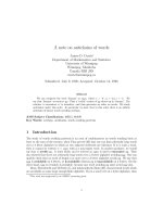
Figure 1: A b-trie with b = 3 built from the following ten strings: X
1
= 11000 ,
X

2
= 11100 , X
3
= 11111 ,andX
4
= 1000 , X
5
= 10111 , X
6
= 10101 ,
X
7
= 00000 , X
8
= 00111 , X
9
= 00101 , X
4
= 00100
There are many possible variations of the trie. One such variation is the b-trie in which
aleafisallowedtoholdasmanyasb strings (cf. [5, 9, 11, 17]). In Figure 1 we show
an example of a 3-trie constructed over n =10strings. Theb-trie is particularly useful
in algorithms for extendible hashing in which the capacity of a page or other storage unit
is b. Also, in lossy compression based on an extension of Lempel-Ziv lossless schemes (cf.
[10, 18]), b-tries (or more precisely, b-suffix trees [17]) are very useful. In these applications,
the parameter b is quite large, and may depend on n. There are other applications of b-tries
in computer science, communications and biology. Among these are partial match retrieval
of multidimensional data, searching and sorting, pattern matching, conflict resolution algo-
rithms for broadcast communications, data compression, coding, security, genes searching,
DNA sequencing, and genome maps.

In this paper, we consider b-tries with a large parameter b, that may depend on n. Such
a tree is built over n randomly generated strings of binary symbols. We assume that every
symbol is equally likely, thus the strings are emitted by an unbiased memoryless source. Our
interest lies in establishing the asymptotic distribution of the height, which is the longest
path in such a b-trie. We also compare our results to those for b-tries with fixed b (cf.
[4, 7, 6, 14]), PATRICIA tries (cf. [7, 9, 11, 13]) and digital search trees (cf. [8, 9, 11]).
We now briefly summarize our main results. We obtain asymptotic expansions of the
distribution Pr{H
n
≤ k} of the height H
n
for five ranges of n, k,andb (cf. Theorem 2).
This should be compared to three regions of n and k for fixed b (cf. Theorem 1). We shall
prove that in the region where most of the probability mass is concentrated, the height
the electronic journal of combinatorics 7 (2000), #R39 3
distribution can be approximated by (for fixed large k and n, b →∞)
Pr{H
n
≤ k}∼exp

−
2
k
√
2π
e
−a
2
/2
a


where a =
√
b(1 − n2
−k
) →∞(cf. Theorem 2 and the Appendix). This resembles an
exponential of a Gaussian distribution. However, a closer look reveals that the asymptotic
distribution of the height is concentrated (for fixed large n and k, b →∞)onthepoint
k
1
= log
2
(n/b) +1, thatis, Pr{H
n
= k
1
} =1− o(1). This should be contrasted with
the height distribution of b-tries with fixed b, in which cases the limiting distribution is of
extreme value type, and is concentrated around (1+1/b)log
2
n. We observe that the height
distribution of b-tries with large b resembles the height distribution for a PATRICIA trie
(cf. [7, 13, 17]). In fact, in [13, 17] the probabilistic behavior of the PATRICIA height was
obtained through the height of b-tries after taking the limit with b →∞.
With respect to previous results, Flajolet [4], Devroye [2], Jacquet and R´egnier [6], and
Pittel [14] established the asymptotic distribution for b-tries with fixed b using probabilistic
and analytic tools (cf. also [7]). To the best of our knowledge, there are no reported results
in literature for large b.
The paper is organized as follows. In the next section we present and discuss our main
results for b-tries for large b (cf. Theorem 2). The proof is delayed until Section 3. It is

based on an asymptotic evaluation of a certain integral.
2 Summary of Results
We let H
n
betheheightofab-trie of size n. We denote its probability distribution by
h
k
n
= Pr{H
n
≤ k}. (2.1)
This function satisfies the non-linear recurrence
h
k
n
=
n

i=0

n
i

2
−n
h
k−1
i
h
k−1

n−i
,k≥ 1 (2.2)
with the initial condition
h
0
n
=1,n=0, 1, ,b; (2.3)
h
0
n
=0,n>b. (2.4)
By using exponential generating functions, we can easily solve (2.2) and (2.3)-(2.4).
Indeed, let us define H
k
(z)=

n≥0
h
k
n
z
n
n!
. Then, (2.2) implies that
H
k
(z)=

H
0

(z2
−k
)

2
k
with H
0
(z)=1+z+···+z
b
/b!. By Cauchy’s formula, we obtain the following representation
of h
k
n
as a complex contour integral:
h
k
n
=
n!
2πi

z
−n−1

1+z2
−k
+
z
2

4
−k
2!
+ ···+
z
b
2
−bk
b!

2
k
dz. (2.5)
the electronic journal of combinatorics 7 (2000), #R39 4
Here the loop integral is around any closed loop about the origin.
To gain more insight into the structure of this probability distribution, it is useful to
evaluate (2.5) in the asymptotic limit n →∞. In [4] and [7] asymptotic formulas were
presented that apply for n large with b fixed, for various ranges of k. For purposes of
comparison, we repeat these results below.
Theorem 1 The distribution of the height of b-tries has the following asymptotic expan-
sions for fixed b:
(i) Right-Tail Region: k →∞, n = O(1):
Pr{H
n
≤ k} =
¯
h
k
n
∼ 1 −

n!
(b +1)!(n −b − 1)!
2
−kb
.
(ii) Central Regime: k, n →∞with ξ = n2
−k
, 0 <ξ<b:
¯
h
k
n
∼ A(ξ; b)e
nφ(ξ;b)
,
where
φ(ξ; b)=−1 − log ω
0
+
1
ξ

b log(ω
0
ξ) − log b! −log

1 −
1
ω
0


,
A(ξ; b)=
1

1+(ω
0
− 1)(ξ −b)
.
In the above, ω
0
= ω
0
(ξ; b) is the solution to
1 −
1
ω
0
=
(ω
0
ξ)
b
b!

1+ω
0
ξ +
ω
2

0
ξ
2
2!
+ ···+
ω
b
0
ξ
b
b!

.
(iii) Left-Tail Region: k,n →∞with j = b2
k
− n
¯
h
k
n
∼
√
2πn
n
j
j!
b
n
exp


−(n + j)

1+b
−1
log b!

where j = O(1).
We also observed that the probability mass is concentrated in the central region when
ξ → 0. In particular,
Pr{H
n
≤ k}∼A(ξ)e
nφ(ξ)
∼ exp

−
nξ
b
(b +1)!

,ξ→ 0
=exp

−
n
1+b
2
−kb
(b +1)!


. (2.6)
In fact, most of the probability mass is concentrated around k =(1+1/b)log
2
n + x where
x is a fixed real number. More precisely:
Pr{H
n
≤ (1 + 1/b)log
2
n + x} = Pr{H
n
≤(1 + 1/b)log
2
n + x}
∼ exp

−
1
(1 + b)!
2
−bx+b(1+b)/b·log
2
n+x

, (2.7)
the electronic journal of combinatorics 7 (2000), #R39 5
where x is the fractional part of x,thatis,x = x −x. Due to the term log
2
n the
limit of (2.7) does not exit as n →∞.

We next consider the limit b →∞. We now find that there are five cases of (n, k)to
consider, and we summarize our final results below. The necessity of treating the five cases
in Theorem 2 is better understood by viewing the problem as first fixing k and b,andthen
varying n (cf. Section 4).
Theorem 2 For b →∞the distribution of the height of b-tries has the following asymptotic
expansions:
(a) b, k →∞, (n −b)2
−k
→ 0, b ≥ δn (δ>0)
1 − h
k
n
=

n
b +1

2
−kb

1+O

n − b −1
2
k

.
(b) b, n, k →∞, (n −b)2
−k
→∞, nb

−1
2
−k
≤ δ
1
< 1
1 − h
k
n
=

n
b

(1 −2
−k
)
n−b
2
k(b−1)

b2
k
n − b
− 1

−1
[1 + O(b(n −b)
−2
4

k
)+O(2
−k
)]
(c) b, n, k →∞, 2
k
= O(
√
b), a ≡
√
b(1 −n2
−k
/b) fixed
h
k
n
=
K
0

1 − a(a + ζ
0
)
exp(2
k
Ψ
0
)

1+O


1
√
b

where
K
0
=exp

2
k
6
√
b
(a + ζ
0
)(a
2
− aζ
0
+4)

,
Ψ
0
=
1
2
(a + ζ

0
)
2
+logQ(ζ
0
)
Q(ζ
0
)=
1
√
2π

∞
ζ
0
e
−x
2
/2
dx,
and ζ
0
= ζ
0
(a) is the solution to the transcendental equation
a + ζ
0
=
e

−ζ
2
0
/2
√
2πQ(ζ
0
)
.
(d) b, n, k →∞with b −n2
−k
= γ fixed
h
k
n
=

b
γ(1 + γ)

1
√
2πb

2
k
e
2
k
ϕ(γ)

[1 + O(b
−1
)]
ϕ(γ)=γ log

1+
1
γ

+log(1+γ).
(e) b, n, k →∞with b2
k
− n = j fixed,
h
k
n
=
√
2πb2
k

1
√
2πb

2
k
2
kj
j!

[1 + O(2
−k
j
2
)]
for j ≥ 0.
the electronic journal of combinatorics 7 (2000), #R39 6
We observe that for cases (c), (d) and (e), h
k
n
is exponentially small, while for cases (a)
and (b), 1 − h
k
n
is exponentially small. From the definition of ζ
0
in part (c), we can easily
show that
ζ
0
(a)=−a +
1
√
2π
e
−a
2
/2
+ O(e
−a

2
),a→ +∞ (2.8)
ζ
0
(a)=
1
a
− 2a + O(a
3
),a→ 0
+
. (2.9)
We also note that from the definition of a b-trie we have h
k
n
=0forn>b2
k
and h
k
n
=1for
0 ≤ n ≤ b, k ≥ 0.
The asymptotic formula for h
k
n
in the matching region between (b) and (c) may be
obtained by evaluating (c) in the limit a →∞. Using (2.8) we are led to (see the Appendix
for the derivation)
h
k

n
∼ exp

−
2
k
√
2π
e
−a
2
/2
a

. (2.10)
This result applies to the limit where b, n, k →∞with a =
√
b(1 − n2
−k
/b) →∞but
n2
−k
/b → 1
−
. Observe that (2.10) asymptotically matches with the result in Theorem
2(b), if a is sufficiently large so that 2
k
e
−a
2

/2
a
−1
→ 0. We note that for fixed large n the
condition a = O(1), with 0 <a<∞,asb →∞may not be satisfied for any k. However,
for fixed large b and k, we can clearly find n so that a =
√
b(1 − n2
−k
/b)=O(1) for some
range of n (see also numerical studies in Section 4). The expansion (2.10) applies when n, b
and k are such that h
k
n
is neither close to 0 nor to 1.
The result (2.10) has roughly the form of an exponential of a Gaussian, and it should
be contrasted with the double exponential in (2.6), which applies for b fixed. The large b
result is somewhat similar to the corresponding one for PATRICIA trees analyzed by us in
[7] and digital search trees discussed in [8].
Next, we apply Theorem 2 for a fixed (large) b and let n and k vary. We first define
k
0
= log
2
(n/b),
and note that h
k
n
=0fork<k
0

. We furthermore set
k = log
2
(n/b)+  =log
2
(n/b)+ −β
where β = log
2
(n/b) (as before · denotes the fractional part). If n/b is a power of 2 then
β = 0 and for  = 0 part (e) of Theorem 2 yields (with j =0)
h
k
0
n
∼
√
2
k
0

1
√
2πb

2
k
0
−1
, 2
k

0
= n/b
which is asymptotically small. On the other hand if β =0and =1then
a =
√
b(1 −n2
−k
/b)=
√
b(1 −2
β−1
)=
1
2
√
b
which is large, so that h
k
0
+1
n
∼ 1. This shows that when n/b is a power of 2, all the mass
accumulates at k
0
+1=log
2
(n/b)+1.
the electronic journal of combinatorics 7 (2000), #R39 7
When n/b is not a power of 2 (with  =1, 2, ) and we consider a fixed β (0 <β<1),
then we can easily show that j, γ and a are all asymptotically large, so that parts (c)-(e)

of Theorem 2 do not apply, and we must use part (b) (or the intermediate result in (2.10))
to compute h
k
n
.Wethushaveh
k
0
−1
n
=0andh
k
0
n
∼ 1 so that the mass accumulates at
k = k
0
= log
2
(n/b)+ 1. In passing we should point out that if we consider a sequence of
n, b such that β → 1
−
, then the conditions where parts (c) and (d) of Theorem 2 are valid
may be satisfied.
We summarize this analysis in the following corollary.
Corollary 1 For any fixed 0 ≤ β<1 and n, b →∞, the asymptotic distribution of the
b-trie height is concentrated on the one point k
1
= log
2
(n/b)+1, that is,

Pr{H
n
= k
1
} =1− o(1)
as n →∞.Ifβ → 1
−
in such a way that 2
k
e
−a
2
/2
a
−1
is bounded, then the height distribution
concentrates on two consecutive points.
3 Derivation of Results
We establish the five parts of Theorem 2. Since the analysis involves a routine use of the
saddle point method (cf. [1, 12]), we only give the main points of the calculations.
The distribution h
k
n
= Pr{H
n
≤ k} is given by the Cauchy integral (2.5). Observe that
1+z2
−k
+ ···+
z

b
2
−kb
b!
= e
z2
−k

∞
z2
−k
e
−w
w
b
b!
dw = e
z2
−k

1 −

z2
−k
0
e
−w
w
b
b!

dw

. (3.1)
It will thus prove useful to have the asymptotic behavior of the integral(s) in (3.1), and this
we summarize below.
Lemma 1 We let
I = I(A, b)=
1
b!

A
0
e
b log w−w
dw =
e
−b
b
b+1
b!

A/b
0
e
b(log u−u+1)
du.
Let α = b/A. Then, the asymptotic expansions of I are as follows:
(i) b, A →∞, α = b/A > 1
I = e
−A

A
b
b!

1
b/A − 1
−
b
A
2
1
(b/A − 1)
3
+ O(A
−2
)

.
(ii) b, A →∞, b/A < 1
I =1−e
−A
A
b
b!

1
1 − b/A
−
b
A

2
1
(1 −b/A)
3
+ O(A
−2
)

.
(iii) b, A →∞, A − b =
√
bB, B = O(1)
I =
1
√
2π


B
−∞
e
−x
2
/2
dx −
1
3
√
b
(B

2
+2)e
−B
2
/2
+
1
b

−
B
5
18
−
B
3
36
−
B
12

e
−B
2
/2
+ O(b
−3/2
)

.

the electronic journal of combinatorics 7 (2000), #R39 8
Proof. ToestablishLemma1wenotethatI is a Laplace-type integral [1, 12]. Setting
f(u)=logu − u + 1 we see that f is maximal at u =1. ForA/b < 1wehavef

(u) > 0
for 0 <u≤ A/b and thus the major contribution to the integral comes from the upper
endpoint (more precisely, from u = A/b − O(b
−1
)). Then, the standard Laplace method
yields part (i) of the Lemma 1. If A/b > 1wewrite

A/b
0
(···)=

∞
0
(···)−

∞
A/b
(···), evaluate
the first integral exactly and use Laplace’s method on the second integral. Now f

(u) < 0
for u ≥ A/b and the major contribution to the second integral is from the lower endpoint.
Obtaining the leading two terms leads to (ii) in the Lemma 1.
To derive part (iii), we scale A −b =
√
bB to see that the main contribution will come

from u − 1=O(b
−1/2
). We thus set u =1+x/
√
b and obtain
I =
e
−b
b
b+1
b!

B
−
√
b
exp

b

log

1+
x
√
b

−
x
√

b

dx
√
b
(3.2)
=
b
b
√
be
−b
b!

B
−∞
e
−x
2
/2

1+
x
3
3
√
b
+
1
b


−
x
4
4
+
x
6
18

+ O(b
−3/2
)

dx.
Evaluating explicitly the integrals in (3.2) and using Stirling’s formula in the form b!=
√
2πbb
b
e
−b
(1 + (12b)
−1
+ O(b
−2
)), we obtain part (iii) of the Lemma.
We return to (2.5) and first consider the limit b →∞with (n −b −1)2
−k
→ 0. Now we
have

2
k
log

1 −

z2
−k
0
e
−w
w
b
b!
dw

∼−
z
b+1
(b +1)!
2
−kb
whichwhenusedin(2.5)yields
1 − h
k
n
=
n!
2πi


e
z
z
n+1

1 − exp

2
k
log

1 −

z2
−k
0
e
−w
w
b
b!
dw

dz
=
n!
2πi

e
z

z
b−n
2
−kb
(b +1)!
(1 + O(z2
−k
))dz
=
n!
(n − b − 1)!
2
−kb
(b +1)!
(1 + O((n − b −1)2
−k
)).
and we obtain part (a) of Theorem 2.
Now consider the limit where (n − b)2
−k
→∞and nb
−1
2
−k
≤ δ
1
< 1. Using Lemma
1(i) we obtain
1 − h
k

n
=
n!
2πi

|z|=(n−b)/(1−2
−k
)
e
z
z
n+1
2
k
e
−z2
−k z
b
2
kb
b!
1
b2
k
/z −1
[1 + O(bz
−2
4
k
)]dz. (3.3)

The above has a saddle where
d
dz
[z +(b −n)logz]=0⇒ z = n − b
and then the standard saddle point approximation to (3.3) yields
1 − h
k
n
∼
n!
(n − b)!b!
(1 −2
−k
)
n−b
2
k(b−1)

b2
k
n − b
− 1

−1
. (3.4)
the electronic journal of combinatorics 7 (2000), #R39 9
We have thus obtained Theorem 2 part (b). The error term therein follows from (3.3).
We proceed to analyze the left tail of the distribution. First, we consider the limit
b, n, k →∞with b2
k

−n = j fixed, and j ≥ 0. We use part (ii) of Lemma 1 to approximate
(3.1). Thus,
z +2
k
log


∞
z2
−k
e
−w
w
b
b!
dw

=2
k
b log(z2
−k
) − 2
k
log(b!) (3.5)
− 2
k
log

1 −
b

z2
−k

+ O(b8
k
z
−2
).
We furthermore scale z =4
k
bt and then (2.5) with (3.5) becomes
h
k
n
= n!e
−2
k
log(b!)
e
2
k
b log(2
−k
)
1
2πi

z
j−1
exp


−2
k
log

1 −
b
z2
−k

[1 + O(b8
k
z
−2
)]dz
= n!(4
k
b)
j
e
−2
k
log(b!)
e
2
k
b log(2
−k
)
1

2πi

t
j−1
e
1/t
[1 + O(2
−k
b
−1
t
−2
+2
−k
t
−2
)]dt
=
n!
j!
(4
k
b)
j
e
−2
k
log(b!)
e
2

k
b log(2
−k
)
[1 + O(j
2
2
−k
)]. (3.6)
Using Stirling’s formula to approximate n!andb! and replacing n by b2
k
− j,wesee
that (3.6) is asymptotically equivalent to Theorem 2(e).
Next we take b, n, k large with b −n2
−k
= γ fixed. We may still use the approximation
(3.5). We now set z =2
k
bτ and obtain from (2.5) and (3.5)
h
k
n
= n!

1
2
k
b

n−2

k
b
e
−2
k
log(b!)

1
2
k

2
k
b
J (3.7)
J =
1
2πi

e
(2
k
b−n)logτ−2
k
log(1−1/τ )
dτ
τ
[1 + O(b
−1
)].

The integral J is easily evaluated by the saddle point method. The saddle point equation
is
d
dτ
[(2
k
b −n)logτ − 2
k
log(1 −1/τ)] = 0
so there is a saddle at τ = τ
0
≡ 1+1/(b − n2
−k
)=1+1/γ. Then the standard leading
order estimate for J is
J ∼
1
√
2π
exp

(2
k
b − n)log

1+
1
γ

+2

k
log(1 + γ)

1

(2
k
b − n)(1 + b − n2
−k
)
. (3.8)
Using (3.8) in (3.7) along with Stirling’s formula, and writing the result in terms of b, k and
γ, we obtain Theorem 2(d).
Finally we consider b, n, k large with a =
√
b(1 −n2
−k
/b) fixed. Now we must use part
(iii) of Lemma 1 to approximate the integrand in (2.5). Setting B =(z2
−k
− b)/
√
b and
using Lemma 1(iii) we obtain
the electronic journal of combinatorics 7 (2000), #R39 10
log(1 − I)=log

1
√
2π


∞
B
e
−x
2
/2
dx −
1
√
2π
B
2
+2
3
√
b
e
−B
2
/2
+ O(b
−1
)

(3.9)
=log

1
√

2π

∞
B
e
−x
2
/2
dx

+
B
2
+2
3
√
b
e
−B
2
/2

∞
B
e
−x
2
/2
dx
+ O(b

−1
).
Setting ζ =(z2
−k
− b)/
√
b we find that
n!e
z
z
−n
=exp

2
k
(b +
√
bζ) − n log(2
k
b) − n log

1+
ζ
√
b

n! (3.10)
=
√
2πn exp


2
k
(a + ζ)
2
2
+
2
k
√
b

a
3
6
−
aζ
2
−
ζ
3
3

+ O

2
k
b

.

Here we have again used Stirling’s formula and recalled that n =2
k
b(1 − a/
√
b). Using
(3.9) and (3.10), (2.5) becomes
h
k
n
=
√
2πn
2πi
1
√
b

K(ζ; b)e
2
k
Ψ(ζ)
dζ (3.11)
where
Ψ(ζ)=
1
2
(a + ζ)
2
+log


1
√
2π

∞
ζ
e
−x
2
/2
dx

and
K(ζ; b)=exp

2
k
√
b

a
3
6
−
aζ
2
2
−
ζ
3

3
+
(ζ
2
+2)e
−ζ
2
/2
3

∞
ζ
e
−x
2
/2
dx

×[1 + O(b
−1/2
, 2
k
b
−1
)].
For k →∞in such a way that a is fixed and 2
k
/b → 0, we evaluate (3.11) by the saddle
point method. The equation locating the saddle points is Ψ


(ζ) = 0, i.e.,
a + ζ =
e
−ζ
2
/2

∞
ζ
e
−x
2
/2
dx
. (3.12)
This defines ζ = ζ
0
(a), which satisfies ζ
0
→−∞as a → +∞ and ζ
0
→ +∞ as a → 0
+
.We
note that n2
−k
/b ∼ 1 and, in view of (3.12),
Ψ

(ζ

0
)=1+
ζ
0
e
−ζ
2
0
/2

∞
ζ
0
e
−x
2
/2
dx
−
e
−ζ
2
0


∞
ζ
0
e
−x

2
/2
dx

2
=1− a
2
− aζ
0
.
Then the standard Laplace estimate of (3.11) leads to part (c) of Theorem 2.
We comment that a more uniform result than that in (c) can be given. We have
h
k
n
∼
n!
√
2π

n
z
2
∗
−
2
−k
1 − I
∗


I

∗
+
(I

∗
)
2
1 − I
∗

−1/2
e
z
∗
z
n+1
∗
(1 −I
∗
)
2
k
(3.13)
the electronic journal of combinatorics 7 (2000), #R39 11
where z
∗
= z
∗

(n, b, k) is the solution to
1 −
n
z
−
I

(z2
−k
; b)
1 − I(z2
−k
; b)
=0,
and I is defined in Lemma 1. Also, I

∗
= I

(z
∗
2
−k
; b)andI

∗
= I

(z
∗

2
−k
; b). The above is
more general than Theorem 2(c) in that the condition 2
k
= O(
√
b) is not required. This
can be obtained by writing
h
k
n
=
n!
2πi

1
z
exp[z − n log z +2
k
log(1 −I(z2
−k
; b))]dz
and using the saddle point method, without using Lemma 1 to approximate I. The saddle
point equation is
d
dz
[z − n log z +2
k
log(1 −I)] = 1 −

n
z
−
I

1 − I
=0
and we ultimately obtain (3.13).
4 Numerical Studies
We determine the numerical accuracy of the results in Theorem 2, and also demonstrate
the necessity of treating the five different scales. To do so, it is best to fix b and k,and
vary n. We consider the range b +1≤ n ≤ b2
k
, since otherwise h
k
n
=1orh
k
n
=0. Wenote
that as we increase n, we gradually move from case (a) to case (e) of Theorem 2. We also
comment that for a fixed large b and n, the conditions under which (c)–(e) apply may not
be satisfied for any k. However, for a fixed large b and k, we can always find a range of n
such that each of the parts of Theorem 2 apply.
In Table 1 we consider b =16andk =2.Wethushave2
k
=
√
b so that the condition
2

k
= O(
√
b), which appears in part (c), is (numerically) satisfied. Table 1 gives the exact
values of 1 −h
k
n
and the approximations from Theorem 2, parts (a) and (b). The part (a)
approximation is denoted by 1 − h
k
n
(a), etc. We see that when n = 17, (a) is a better
approximation than (b), but (b) is superior when n ≥ 18.
InTable2weretainb =16andk = 2, but now take 46 ≤ n ≤ 64. We tabulate the
exact h
k
n
along with the asymptotic results in parts (c)–(e) of Theorem 2. We also give the
corresponding values of a =
√
b(1 − n2
−k
/b), γ = b − n2
−k
and j = b2
k
− n, since these
results assume that a, γ and j are O(1), respectively. When n = 64, approximation (e)
is accurate to within 2%. When n = 63, (e) is more accurate than (d), but (d) becomes
superior for n ≤ 62. When n is further decreased to n = 54, (c) becomes more accurate

than (d). We also recall that when h
k
n
is not close to either 0 or 1, then part (c) applies.
In Tables 3 and 4 we increase b and k to b =64andk = 3 (thus retaining 2
k
=
√
b). In
Table 3 we consider 1 −h
k
n
for cases (a) and (b) and in Table 4 we give h
k
n
for cases (c)–(e)
(again tabulating the values of a, γ and j). When n =65=b + 1, (a) is superior to (b),
but (b) is the better approximation for n ≥ 66. Table 4 considers 400 ≤ n ≤ 512 = b2
k
and
demonstrates the transition between cases (c) and (d) and then (d) and (e). In general,
the results in Tables 3 and 4 are more accurate than those in Tables 1 and 2, as one would
expect, since the asymptotics apply for b →∞.
the electronic journal of combinatorics 7 (2000), #R39 12
Table 1: b = 16, k =2
n 1 − h
k
n
(exact) 1 − h
k

n
(a) 1 − h
k
n
(b)
17 .233 (10
−9
) .233 (10
−9
) .188 (10
−9
)
18 .320 (10
−8
) .419 (10
−8
) .259 (10
−8
)
19 .232 (10
−7
) .398 (10
−7
) .187 (10
−7
)
20 .118 (10
−6
) .265 (10
−6

) .951 (10
−7
)
21 .475 (10
−6
) .139 (10
−5
) .381 (10
−6
)
22 .160 (10
−5
) .613 (10
−5
) .128 (10
−5
)
23 .469 (10
−5
) .374 (10
−5
)
24 .123 (10
−4
) .980 (10
−5
)
26 .652 (10
−4
) .516 (10

−4
)
28 .263 (10
−3
) .207 (10
−3
)
30 .863 (10
−3
) .676 (10
−3
)
32 .240 (10
−2
) .187 (10
−2
)
34 .585 (10
−2
) .453 (10
−2
)
36 .127 (10
−1
) .139 (10
−2
)
38 .253 (10
−1
) .194 (10

−1
)
40 .462 (10
−1
) .352 (10
−1
)
42 .790 (10
−1
) .599 (10
−1
)
44 .127 .958 (10
−1
)
46 .193 .146
48 .278 .211
50 .383 .294
Table 2: b = 16, k =2
n h
k
n
(exact) (a) h
k
n
(c) (γ) h
k
n
(d) (j) h
k

n
(e)
46 .807 (1.125) .960
48 .722 (1.000) .873
50 .617 (.875) .763
52 .497 (.750) .635
54 .370 (.563) .497 (2.50) .581
56 .247 (.500) .359 (2.00) .335
58 .142 (.375) .238 (1.50) .171
60 .643 (10
−1
) (1.00) .716 (10
−1
)
61 .378 (10
−1
) (.75) .412 (10
−1
) (3) .211 (10
−1
)
62 .193 (10
−1
) (.50) .208 (10
−1
) (2) .159 (10
−1
)
63 .778 (10
−2

) (.25) .864 (10
−2
) (1) .794 (10
−2
)
64 .195 (10
−2
) (0) .198 (10
−2
)
the electronic journal of combinatorics 7 (2000), #R39 13
Table 3: b = 64, k =3
n 1 − h
k
n
(exact) 1 − h
k
n
(a) 1 − h
k
n
(b)
65 .159 (10
−57
) .159 (10
−57
) .142 (10
−57
)
66 .922 (10

−56
) .105 (10
−55
) .821 (10
−56
)
67 .271 (10
−54
) .352 (10
−54
) .241 (10
−54
)
68 .538 (10
−53
) .798 (10
−53
) .479 (10
−53
)
69 .814 (10
−52
) .138 (10
−51
) .724 (10
−52
)
70 .100 (10
−50
) .193 (10

−50
) .889 (10
−51
)
100 .176 (10
−32
) .156 (10
−32
)
150 .564 (10
−19
) .492 (10
−19
)
200 .118 (10
−11
) .102 (10
−11
)
250 .468 (10
−7
) .395 (10
−7
)
300 .522 (10
−4
) .431 (10
−4
)
350 .583 (10

−2
) .468 (10
−2
)
400 .130 .103
Table 4: b = 64, k =3
n h
k
n
(exact) (a) h
k
n
(c) (γ) h
k
n
(d) (j) h
k
n
(f)
400 .870 (1.75) .924
420 .690 (1.44) .743
440 .416 (1.13) .454
460 .145 (.81) .164
480 .166 (10
−1
) (.48) .204 (10
−1
) (4) .337 (10
−1
)

500 .980 (10
−4
) (.17) .202 (10
−3
) (1.50) .111 (10
−3
)
508 .702 (10
−6
) (.500) .733 (10
−6
) (5) .370 (10
−6
)
509 .256 (10
−6
) (.375) .268 (10
−6
) (4) .185 (10
−6
)
510 .772 (10
−7
) (.250) .816 (10
−7
) (2) .694 (10
−7
)
511 .172 (10
−7

) (.125) .188 (10
−7
) (1) .174 (10
−7
)
512 .215 (10
−8
) (0) .217 (10
−8
)
the electronic journal of combinatorics 7 (2000), #R39 14
These data also suggest that in some cases it may be desirable to calculate some of
the higher order terms in the asymptotic series. For case (c) these are likely to be of
order O(b
−1/2
) relative to the leading term, for 2
k
= O(
√
b). The overall accuracy of the
asymptotic results is also consistent with O(b
−1/2
) error terms. Finally, we comment that
by calculating higher order terms in the expansions in Lemma 1, it may be possible to relax
the condition 2
k
= O(
√
b), that appears in some part (c) of Theorem 2 (see also (3.13)).
ACKNOWLEDGMENT: We thank the referee for useful suggestions.

Appendix
We discuss the asymptotic matching region between cases (b) and (c) of Theorem 2. In par-
ticular, we establish (2.10) in the matching region directly from the integral representation
(2.5).
We use an approximation to I that applies for A −b = o(b) but with (A−b)/
√
b = B →
−∞. In this range we have, from Lemma 1,
1 − I ∼ 1 −
e
−B
2
/2
√
2π

1
B
−
B
2
3
√
b
+ ···

and hence
h
k
n

∼
n!
2πi

e
z
z
n+1

1+
e
−B
2
/2
B
√
2π

1 −
B
3
3
√
b
+ ···

2
k
dz
∼

n!
2πi

e
2
k
b
e
2
k
√
bB
√
b2
−kn
(b +
√
bB)
n+1
exp

e
−B
2
/2
B
2
k
√
2π


1 −
B
3
3
√
b

dB. (A.1)
Next we use
exp(2
k
√
bB)

1+
B
√
b

−n
∼ exp

2
k
√
b −
n
√
b


B +
n
2b
B
2

=exp

2
k

aB +
n
2
k
b
B
2
2

in (A.1) and note that in the matching region n/(2
k
b) ∼ 1. We recall that a =
√
b(1 −
n2
−k
/b).
The integrand in (A.1) has a saddle point at B = −a and a standard application of the

steepest descent method yields
h
k
n
∼
n!
b
n
√
b
e
2
k
b
1
√
2π
2
−kn
2
−k/2
e
−2
k
a
2
/2
exp

−

e
−a
2
/2
a
√
2π
2
k

. (A.2)
But in this limit we have
n!
b
n
e
2
k
b
2
−kn
∼

n
b2
k

n
√
2πne

2
k
b−n
the electronic journal of combinatorics 7 (2000), #R39 15
=
√
2πn

1 −
a
√
b

n
e
2
k
√
ba
∼
√
2πn exp

2
k
√
b −
n
√
b


a −
n
2b
a
2

∼
√
2πb2
k/2
exp

2
k
a
2
2

.
Using the above in (A.2) establishes (2.10) and shows that there are no “gaps” in the
asymptotics between cases (b) and (c).
References
[1] N. Bleistein and R. Handelsman, Asymptotic Expansions of Integrals, Dover Publica-
tions, New York 1986.
[2] L. Devroye, A Probabilistic Analysis of the Height of Tries and the Complexity of Trie
Sort, Acta Informatica, 21, 229–237, 1984.
[3] L. Devroye, A Study of Trie-Like Structures Under the Density Model, Ann. Appl.
Probability, 2, 402–434, 1992.
[4] P. Flajolet, On the Performance Evaluation of Extendible Hashing and Trie Searching,

Acta Informatica, 20, 345–369, 1983.
[5] D. Gusfield, Algorithms on Strings, Trees, and Sequences, Cambridge University Press,
1997.
[6] P. Jacquet and M. R´egnier, Trie Partitioning Process: Limiting Distributions, Lecture
Notes in Computer Science, 214, 196-210, Springer Verlag, New York 1986.
[7] C. Knessl and W. Szpankowski, Limit Laws for Heights in Generalized Tries and PA-
TRICIA Tries, Proc. LATIN’2000, Punta del Este, Uruguay, Lecture Notes in Com-
puter Science, 1776, 298-307, 2000.
[8] C. Knessl and W. Szpankowski, Asymptotic Behavior of the Height in a Digital Search
Tree and the Longest Phrase of the Lempel-Ziv Scheme, SIAM J. Computing, 2000.
[9] D. Knuth, The Art of Computer Programming. Sorting and Searching, Second Edition,
Addison-Wesley, 1998.
[10] T. Luczak and W. Szpankowski, A Suboptimal Lossy Data Compression Based in Ap-
proximate Pattern Matching, IEEE Trans. Information Theory, 43, 1439–1451, 1997.
[11] H. Mahmoud, Evolution of Random Search Trees, John Wiley & Sons, New York 1992.
[12] A. Odlyzko, Asymptotic Enumeration, in Handbook of Combinatorics,Vol.II,(Eds.R.
Graham, M. G¨otschel and L. Lov´asz), Elsevier Science, 1063-1229, 1995.
the electronic journal of combinatorics 7 (2000), #R39 16
[13] B. Pittel, Asymptotic Growth of a Class of Random Trees, Ann. of Probab., 13, 414–
427, 1985.
[14] B. Pittel, Path in a Random Digital Tree: Limiting Distributions, Adv. Appl. Prob.,
18, 139–155, 1986.
[15] M. R´egnier, On the Average Height of Trees in Digital Searching and Dynamic Hashing,
Inform. Processing Lett., 13, 64–66, 1981.
[16] W. Szpankowski, On the Height of Digital Trees and Related Problems, Algorithmica,
6, 256–277, 1991.
[17] W. Szpankowski, A Generalized Suffix Tree and its (Un)Expected Asymptotic Behav-
iors, SIAM J. Computing, 22, 1176-1198, 1993.
[18] E.H. Yang, and J. Kieffer, On the Performance of Data Compression Algorithms Based
upon String Matching, IEEE Trans. Information Theory, 44, 47-65, 1998.