Báo cáo toán học: "Parking functions, empirical processes, and the width of rooted labeled trees" pps
Bạn đang xem bản rút gọn của tài liệu. Xem và tải ngay bản đầy đủ của tài liệu tại đây (214.42 KB, 19 trang )
Parking functions, empirical processes,
and the width of rooted labeled trees
Philippe Chassaing
Institut Elie Cartan
Vandoeuvre, France
Jean-Fran¸cois Marckert
Universit´e de Versailles St-Quentin en Yvelines
Versailles, France
Submitted: August 31, 1999; Accepted: February 8, 2001.
MR Subject Classifications: 05C05, 60J65, 60J80, 62G30
Abstract
This paper provides tight bounds for the moments of the width of rooted labeled
trees with n nodes, answering an open question of Odlyzko and Wilf (1987). To this
aim, we use one of the many one-to-one correspondences between trees and parking
functions, and also a precise coupling between parking functions and the empirical
processes of mathematical statistics. Our result turns out to be a consequence of the
strong convergence of empirical processes to the Brownian bridge (Koml´os, Major
and Tusn´ady, 1975).
Key words. Rooted labeled trees, moment, width, Brownian excursion, empirical
processes, hashing with linear probing, parking.
1 Introduction
An order
n
+1
labeled tree
is a connected graph with set of vertices
{
0
,
1
,
2
,
3
, , n}
,and
with
n
edges. If we specify one vertex to be the root, we have a
rooted
labeled tree.
According to Cayley (1889) the number of such trees is (
n
+1)
n
.
For
τ
chosen at random in the set of order
n
+ 1 rooted labeled trees, let
G
(n)
k
(
τ
)
denote the number of nodes at distance
k
from the root of
τ
,andlet
H
n
(
τ
)denotethe
maximum distance of a node from the root, the
height
of
τ
;(
G
(n)
k
)
k≥0
is the
profile
of
the tree. The
width W
n
(
τ
) is defined by
W
n
=max
0≤k≤H
n
G
(n)
k
.
the electronic journal of combinatorics
8
(2001), #R14
1
Odlyzko and Wilf (1987) used a Perron-Frobenius-like theory to derive asymptotics
for the cumulative function of W
n
. They also proved that
C
1
√
n ≤ E(W
n
) ≤ C
2
n log n,
and left the first term in the asymptotic of E(W
n
)asanopenquestion.
Let (t) denote the local time of the normalized Brownian excursion e(.)atlevelt,i.e.
(t) = lim
ε→0
+
1
ε
1
0
I
[t,t+ε]
(e(u)) du.
Aldous [1] conjectured that t −→ G
(n)
t
√
n
/
√
n would converge weakly, as a stochastic
process, to t −→ (t)/2. Aldous’s conjecture was settled by Drmota and Gittenberger [9].
As noted by these last authors, their result entails the weak convergence of W
n
/
√
n to the
maximum m of the Brownian excursion, as (t) is itself a Brownian excursion changed of
time [5]. Previously, the weak convergence of W
n
/
√
n to m was proven directly by Tak´acs
(1993).
However weak convergence does not answer completely the question of Odlyzko &
Wilf, as it does not yield convergence of the first moment, and even less the speed of this
convergence. The aim of our paper is to fill this gap. Our proof uses the breadth first
search (BFS) random walk [3, 27], following Tak´acs [28], who used the BFS random walk
to prove convergence of moments of the width for binary trees, or general unlabeled trees,
by a clever use of the ballot theorem. For rooted labeled trees, we need an additional
ingredient: a close connection between rooted labeled trees and empirical processes of
mathematical statistics [26], which, we believe, has interest in itself. For instance, this
connection gives an alternative O(n) algorithm, for the generation of a random rooted
labeled tree, to the O(n) algorithm using Pr¨ufer-Knuth’s correspondence (see [16, 20]). It
also allows to analyze the size of parking blocks during the phase transition [7]. Note that
Aldous, or Drmota and Gittenberger’s results are actually about general simple trees.
Rooted labeled trees are a special case of simple trees, but an important one [16, 20].
Recall [5, 8, 15] that the maximum m of the Brownian excursion satisfies
Pr(m ≤ x)=
−∞<k<+∞
(1 −4k
2
x
2
)e
−2k
2
x
2
,
E(m)=
π
2
,
and, for r>1,
E(m
r
)=2
−r/2
r(r −1)Γ
r
2
ζ(r).
We shall say that m is theta-distributed by reference to Jacobi’s Theta function. Inciden-
tally, it is also well known that theta-distributed random variables occur as a limit for
the height of trees: see R´enyi and Szekeres (1967) for rooted labeled trees, Flajolet and
Odlyzko (1982) for general simple trees.
Let us state the main result of this paper:
the electronic journal of combinatorics 8 (2001), #R14 2
Theorem 1.1 For p ≥ 1,
E
n
−p/2
W
p
n
−E(m
p
)=O
p
n
−1/4
log n
.
As a special case,
E(W
n
) −
πn
2
= O
n
1/4
log n
.
One of the motivations of Odlyzko and Wilf, when they study the width of labeled
trees, is to give a tight estimate for the average bandwidth of this class of tree.
2 The breadth first search random walk
From now on, we assume, without consequences for W
n
(τ)’s distribution, that τ is drawn
at random in the subset Ω
n
of labeled trees rooted at 0. The BFS of the rooted labeled
tree starts with the root, 0, and is implemented by maintaining a queue Q, that is initially
(0). Then, at each of the n following stages of the BFS, the vertex x at the head of the
queue is removed from the queue, and all “new” neighbors of x areaddedattheendof
the queue, in increasing order. At step 0, the search produces the set A
0
of neighbors
4 6
3
8
0
1
25
7
9
1
2
264 5
6 3
3
7
7
8
8 9
5
5
Figure 1: Successive states of the queue.
of vertex 0, so that after step 0 the queue contains exactly the elements of A
0
, but not
0 anymore. At step 1, the search produces the set A
1
of new neighbors of the smallest
element x in A
0
, so that after step 1 the queue contains A
0
∪ A
1
−{x}.LetA
k
denote
the set of new elements in the queue after step k,andlet
a
k
=#A
k
.
A labeled tree τ with vertices {0, 1, 2, 3, , n},rootedat0,isdescribedbyasequence
of disjoint sets (A
i
)
0≤i≤n
,whoseunionis{1,2, , n}, and whose cardinalities a
i
=#A
i
satisfy the following set of constraints
a
0
≥ 1,
the electronic journal of combinatorics 8 (2001), #R14 3
a
0
+ a
1
− 1 ≥ 1,
a
0
+ a
1
+ + a
k
− k ≥ 1, (2.1)
a
0
+ a
1
+ + a
n−1
− n +1 ≥ 1,
a
0
+a
1
+ + a
n
− n =0.
Constraints (2.1) are necessary and sufficient conditions for a tree to be connected, or for
the queue to become empty only after step n.
We call BFS random walk the sequence y
(n)
=
y
(n)
k
(τ)
0≤k≤n
of queue lengths: y
(n)
k
(τ)
denotes the number of vertices in the queue after step k, defined by y
(n)
0
= a
0
and
y
(n)
k
= a
0
+ a
1
+ + a
k
− k,
y
(n)
k
−y
(n)
k−1
= a
k
−1.
The proof of Theorem 1.1 relies on the expression of the profile and of the width of
the tree in term of the BFS random walk: observe that G
(n)
1
= y
(n)
0
, G
(n)
2
= y
(n)
G
(n)
1
. More
generally, at step G
(n)
1
+ G
(n)
2
+ + G
(n)
k
, we explore the last vertex at a distance k from
the root, and the queue contains exactly the vertices at distance k +1fromtheroot,
leading to
G
(n)
k+1
= y
(n)
G
(n)
1
+G
(n)
2
+ +G
(n)
k
.
Actually, this is Kendall’s embedding of a Galton-Watson process in the process of queue
lengths, when studying a single-server queue [23].
Thus W
n
is the maximum of a sample of y
(n)
i
. Due to slow variation of the sequence
(y
(n)
k
)
0≤k≤n
, this sample turns out to be “representative”, in the sense that the maximum
of the sample is close to the maximum of the whole sequence.
Proposition 2.1 For any p ≥ 1
W
n
− max
k
y
(n)
k
p
= O
p
(n
1/4
log n).
The proof is given in the next Section. In Section 4, we use a connection between labeled
trees and empirical processes, more easily explained with the help of parking functions,
to prove the next Proposition.
Proposition 2.2 In some probability space, there exists a sequence m
n
of theta-
distributed random variables and a sequence of copies of y
(n)
such that, for any p ≥ 1,
max
k
y
(n)
k
− m
n
√
n
p
= O
p
(log n).
As a consequence, we have
the electronic journal of combinatorics 8 (2001), #R14 4
4
6
3
8
0
1
2
5
7
9
1
2
264 5
6 3
3
7
7
8
8 9
5
5
(n)
y
k
k
G
k
(n)
k
Figure 2: Embedding of the profile in the BFS random walk.
Proposition 2.3 In some probability space, there exists a sequence m
n
of theta-
distributed random variables and a sequence of copies of W
n
such that, for any p ≥ 1,
W
n
√
n
− m
n
p
= O
p
n
−1/4
(log n)
1/2
.
Then
E
W
n
√
n
p
− E(m
p
)
≤ p max
W
n
√
n
p
, m
p
p−1
W
n
√
n
p
−m
n
p
= O
p
n
−1/4
(log n)
1/2
,
leading to Theorem 1.1.
3 Proof of Proposition 2.1
The number of n-tuples (A
i
)
0≤i≤n
with cardinalities (a
i
)
0≤i≤n
,
n!
a
0
!a
1
! a
n
!
,
is proportional to the product of Poisson probabilities e
−1
/a
i
!, so, if a labeled tree τ,
rooted at 0, is drawn at random, the corresponding sequence (a
i
(τ))
0≤i≤n
has the distri-
bution of independent Poisson random variables with mean value 1, conditioned to satisfy
constraints (2.1) (see Spencer (1997)). In other words, the corresponding unlabeled tree
the electronic journal of combinatorics 8 (2001), #R14 5
is a Galton-Watson tree with Poisson(1) progeny, constrained to have n + 1 nodes, and
A
k
is the progeny of the k
th
node visited by the BFS.
As a consequence, the sequence y
(n)
=(y
(n)
k
)
0≤k≤n
is a random walk with length n and
i.i.d. increments a
i
− 1, conditioned to satisfy (2.1). Set
M
n
=max
k
y
(n)
k
.
The aim of this section is to bound the difference between M
n
and W
n
. Essentially, we
follow the line of proof of [28, formula 63, page 200], but we improve Tak´acs’s bounds
with the help of Petrov’s Theorem 3.2. Let x ∨ y denote the maximum of x and y,and
let Ω
δ
(n)bethesetofsequencesy=(y
k
)
k=0, ,n
that satisfy
|y
m+k
−y
m
|≤δ
log n ∨
k log n
whenever k ≥ 0, m ≥ 0andm+k≤n.Wehave
Proposition 3.1 Given any positive number α there exists a constant κ(α), not de-
pending on n,suchthat
Pr
y
(n)
/∈ Ω
κ(α)
(n)
= o
α
(n
−α
).
Proof. Let (N
k
)
0≤k≤n
be a sequence of independent random variables with mean 1,
Poisson-distributed, and let t =(t
k
)
0≤k≤n
be the random walk with increments N
k
− 1.
Let ∆(n)denotethesetofsamplepathsythat satisfy constraints (2.1). As a consequence
of Spencer’s key remark,
Pr(y/∈Ω
δ
(n)) = Pr(t/∈Ω
δ
(n)|t∈∆(n))
≤
Pr(t/∈Ω
δ
(n))
Pr(t ∈ ∆(n))
.
According to Otter’s formula [23], we have
Pr(t ∈ ∆(n)) =
1
n
Pr(t
n
=0),
so due to the standard local limit theorem [11, Ch. 4, Th. 4.2.1] we obtain
Pr(t ∈ ∆(n)) = Θ(n
−3/2
).
Thus we are to prove Proposition 3.1 only for the unconditioned random walk t, but this
is a consequence of the next Theorem [22, p.52-55].
Theorem 3.2 (Petrov, 1975) Let Y
k
be a random walk with i.i.d. increments X
k
satisfying simultaneously
- E(X
k
)=0, and
the electronic journal of combinatorics 8 (2001), #R14 6
- for some positive constant α, E(e
α|X
k
|
) < +∞,
then:
i) there exists two positive real constants g and T such that
E(exp(λX
1
)) ≤ exp(gλ
2
) for |λ| <T,
ii) for (Y
k
)
k≥1
defined as above, we have
Pr(|Y
k
|≥x) ≤ 2exp
−
x
2
4kg
if 0 ≤ x ≤ kgT,
≤ 2exp
−
Tx
2
if x ≥ kgT.
For δ ≥ gT, Theorem 3.2 yields
Pr(t/∈Ω
δ
(n)) ≤ Pr
∃m, k ||t
m+k
−t
m
|≥δ
log n ∨
k log n
≤ n
n
k=1
Pr
|t
k
|≥δ
log n ∨
k log n
≤ 2n
δ
2
log n
T
2
g
2
k=1
n
−δT/2
+2n
n
k=
δ
2
log n
T
2
g
2
n
−δ
2
/4g
≤
2δ
2
log n
T
2
g
2
n
1−δT/2
+2n
2−δ
2
/4g
.
For δ large enough, the last term is o
α
(n
−α
). ♦
For the end of the proof of Proposition 2.1, recall that G
(n)
i
= y
m(i)
,inwhichm(1) = 0
and m(i +1) = m(i)+G
(n)
i
.Consideranintegerksuch that y
k
= M
n
: for some i,
k ∈ [m
i
,m
i+1
[, so that
0 ≤ M
n
− W
n
≤ M
n
− G
(n)
i
≤ δ
log n ∨
(k −m(i)) log n
I
Ω
δ
(n)
+ n
1 −I
Ω
δ
(n)
≤ δ
log n ∨
G
(n)
i
log n
I
Ω
δ
(n)
+ n
1 − I
Ω
δ
(n)
≤ δ
log n +
M
n
log n
I
Ω
δ
(n)
+ n
1 − I
Ω
δ
(n)
(3.2)
≤ δ
log n +
δ
√
n log
3/2
n
I
Ω
δ
(n)
+ n
1 −I
Ω
δ
(n)
.
Thus, owing to Proposition 3.1, for a suitable choice of δ,
E (|W
n
− M
n
|
p
) ≤ δ
p
log n +
δ
√
n log
3/2
n
p
+ n
p
Pr
y
(n)
/∈ Ω
δ(p)
(n)
= O
p
n
p/4
(log n)
3p/4
.
the electronic journal of combinatorics 8 (2001), #R14 7
This last estimate holds true under hypothesis of finite exponential moments for the
progeny. Actually, to obtain a complete proof of Proposition 2.1, we need to decrease the
exponent of log n from 3p/4top/2. In the special case of labeled trees (Poisson progeny),
we shall prove at the end of the next Section, as a consequence of the DKW inequality
for empirical processes, that
Lemma 3.3 For p ≥ 1, E(M
p/2
n
)=O
p
n
p/4
.
For a suitable choice of δ, relation (3.2) and Lemma 3.3 yield Proposition 2.1.
4 Proof of Proposition 2.2
4.1 Rooted labeled trees and parking functions
As y
(n)
is distributed like a random walk with i.i.d. increments conditioned on first return
to 0 being at time n (cf. (2.1)), it rescales to Brownian excursion:
y
(n)
nt
√
n
0≤t≤1
weakly
−→ ( e ( t ))
0≤t≤1
,
and thus
max
k
y
(n)
k
√
n
weakly
−→ m =max
0≤t≤1
e(t).
Inthissectionweprovethemoredemandingconvergenceofmoments,throughacoupling
labeled trees-empirical processes more easily explained through parking functions.
A first correspondence between parking functions and acyclic functions was discovered
by Sch¨utzenberger (1968). The description of the equivalent connection between labeled
trees rooted at 0 and parking functions, through the BFS random walk, is more convenient
for our purpose. In hashing with linear probing, or parking [13, 17], we consider the case
with n cars and n +1places {0,1,2, , n},carc
k
parking on place p
k
if p
k
is still empty,
that is, if a car with a smaller index did not park on place p
k
before. Otherwise car c
k
tries places (p
k
+1)modn+1,(p
k
+2) modn+ 1, , until it finds an empty place. We
consider parking functions (resp. confined sequences) in the terminology of [14] (resp. of
[13, 17]), that is sequences ω =(p
k
)
1≤k≤n
such that the last empty place is place n. Such
a parking function ω is alternatively characterized by the sequence
˜
A
i
(ω)
0≤i≤n
,where
˜
A
i
(ω)={k |p
k
=i}
is the set of cars whose first try is place i.
Let ˜a
i
(ω)denote#
˜
A
i
(ω), and let ˜y
(n)
k
(ω) denote the number of cars that tried, suc-
cessfully or not, to park on place k.Fork=0,wehave
˜y
(n)
k
=˜y
(n)
k−1
−1+˜a
k
=˜a
0
+˜a
1
+ +˜a
k
−k,
the electronic journal of combinatorics 8 (2001), #R14 8
since either place k − 1 is occupied by car c
i
and, among the ˜y
(n)
k−1
cars that visited place
k −1, only c
i
won’t visit place k,orplacek−1isempty:onlyk−1=n,k= 0, belongs
to this last case, and clearly
˜y
(n)
0
=˜a
0
.
So a sequence (
˜
A
i
)
0≤i≤n
is associated with a confined parking scheme if and only if (˜a
i
)
0≤i≤n
satisfies the constraints (2.1), since a place k isemptyonlyif˜y
(n)
k
(ω)=0.
Finally, observing that each of the (n +1)
n−1
sequences (
˜
A
i
)
0≤i≤n
that satisfies (2.1)
defines simultaneously a unique parking function (confined sequence) ω for n cars on n+1
places and a unique order n + 1 labeled tree τ(ω) rooted at 0, we obtain
Proposition 4.1 There exists a one-to-one correspondence ω → τ(ω) between parking
functions and trees, such that for any k and ω
y
(n)
k
(τ(ω)) = ˜y
(n)
k
(ω).
As a consequence, note that if D(n +1,n) denotes the total displacement of cars, we
have
D(n +1,n)=−n+
n
k=0
y
(n)
k
= −n +(n+1)
3/2
1
0
y
(n)
(n+1)t
√
n +1
dt.
Thus
n
−3/2
D(n +1,n)
weakly
−→
1
0
e ( t ) dt,
and we recover here partly the convergence of moments of the total displacement towards
the moments of the Airy law, already obtained by Flajolet et al. [13]: the Airy law
is known as the law of the area below the Brownian excursion. At Subsection 4.5 we
shall complete this alternative proof with the help of the connection parking functions –
empirical processes.
4.2 Empirical processes
Consider a sequence of independent random variables (U
i
)
i≥1
, each of them uniform on
[0, 1]. Let F
n
(t)denotetheempirical distribution function for (U
i
)
1≤i≤n
,definedfort∈
[0, 1] by
F
n
(t)=
#{i|1≤i≤nand U
i
≤ t}
n
.
We recall a few facts about the convergence of the empirical distribution function towards
the distribution function F (t)=tof the uniform law [26]. The speed of convergence of
many interesting statistics is revealed by the empirical process
α
r
(t)=
√
r(F
r
(t)−F(t)),
that satisfies
the electronic journal of combinatorics 8 (2001), #R14 9
1
2
Ø3 7
4
6
8 ØØ 9
5
Ø
A
0
A
1
A
2
A
3
A
4
A
5
A
6
A
7
A
8
A
9
1
2
264 5
6 3
3
7
7
8
8 9
5
5
0
4
6
3
8
0
1 2
5
7
9
1
2
234 5
6 6
6
7
7
8
8 9
5
5
Figure 3: Correspondence trees ↔ parking.
Theorem 4.2 (Donsker, 1952)
(α
r
(t))
t∈[O,1]
weakly
−→ ( b ( t ))
t∈[O,1]
,
b(t) being the Brownian bridge.
Thus the first error term is of order O(1/
√
r). The second error term is given by the
following Theorem of ”strong convergence”:
Theorem 4.3 (Koml´os, Major & Tusn´ady, 1975) Given U
1
, U
2
, uniform on [0, 1]
and independent, there exists a sequence (b
n
)
n≥1
of Brownian bridges such that for all n
and x,
Pr
sup
0≤t≤1
|α
n
(t) − b
n
(t)|≥
Alog n + x
√
n
≤ Me
−µx
,
where A, M and µ are positive absolute constants.
Equivalently, we can write
F
n
(t)=F(t)+
b
n
(t)
√
n
+
r
n
(t)
n
,
in which r
n
(t) denotes
√
n (α
n
(t) −b
n
(t)), and satisfies
Pr
sup
0≤t≤1
|r
n
(t)|≥Alog n + x
≤ Me
−µx
.
KMT’s Theorem is the last ingredient we need to estimate W
n
p
.
the electronic journal of combinatorics 8 (2001), #R14 10
01
1
F, F
n
71 9 36 8 54 2
U , i=
i
01
α
n
Figure 4: Empirical distribution F
n
, empirical process α
n
.
4.3 Parking functions and empirical processes
Let (U
i
)
1≤i≤n
denote a sequence of i.i.d. random variables, each of them uniform on [0, 1],
and let the first try of car c
i
be at place
p
i
= (n +1)U
i
,
assuming that place n +1isalsoplace0. LetD
i
denote the set of cars whose first try is
place i,setd
i
=#D
i
,andletz
(n)
k
denote the number of cars that tried, successfully or
not, to park on place k.LetV(ω) denote the last empty place.
Compared with Subsection 4.1, we have some changes: the ”parking” functions, or
hashing sequences, ω =(k→p
k
, 0≤k≤n), are not confined anymore, and there are
now (n +1)
n
such functions ω, clearly equiprobable ; V (ω)isnotnanymore: V is now
random uniform on {0, 1, 2, , n}.
Let α
n
be the empirical process of (U
1
,U
2
, , U
n
). We have
the electronic journal of combinatorics 8 (2001), #R14 11
1 23 4
5 5
5
6
6
7
8
89
0
U , i=
i
1
71 9
3
6
8
5
4
2
V
parking, displacements
z
k
(n)
7
Figure 5: BFS random walk associated to (U
1
,U
2
, , U
n
)
Proposition 4.4 The relation
α
n
T (n)
n +1
=min
0≤k≤n
α
n
k
n+1
,
defines a unique number T (n) between 0 and n. Furthermore,
T (n)=V.
As a consequence, T (n) is uniformly distributed on {0, 1, 2, , n}.Also,theempty
place V does not depend on the chronology (the D
i
’s), but only on the sequence (d
i
)
0≤i≤n
,
sincewehave
α
n
k
n+1
=
1
√
n
d
1
+d
2
+ + d
k
− k
n
n +1
.
Proof : Set θ(n, i)=
√
nα
n
(i/n +1). For 0≤i<j≤n+1, θ(n, i)=θ(n, j)can
occur only if (i −j)
n
n+1
is an integer, i.e. if (i, j)=(0,n+ 1), as the fractional parts of
θ(n, j) − θ(n, i)and(i−j)
n
n+1
are the same: the number of cars whose first try belongs
to {i +1,i+2, , j} is given by
d
i+1
+ d
i+2
+ + d
j
= θ(n, j) −θ(n, i) −(i −j)
n
n +1
.
Thus i −→ α
n
(i/n + 1) reaches its minimum only once in {0, 1, 2, , n},andT(n)iswell
defined. For k =1,2, , n +1,wehave
θ(n, V + k) −θ(n, V )=d
V+1
+ d
V +2
+ + d
V +k
− k
n
n +1
= z
(n)
V+k
+k−1−k
n
n+1
= z
(n)
V+k
+
k
n+1
−1, (4.3)
the electronic journal of combinatorics 8 (2001), #R14 12
V
T(n)
U , i=
i
71 9 36 8 54 2
z
k
(n)
α
n
(
t
),
α
n
(
),
k
n+1
Figure 6: The empirical process and the empty place.
the second equality, as already seen in Subsection 4.1, due to the fact that z
(n)
V +1
= d
V +1
,
but for k = V , z
(n)
k+1
= z
(n)
k
− 1+d
k+1
. Finally, for k =1,2, , n, z
(n)
V +k
≥ 1sothelast
term is positive, that is, k → θ(n, k) reaches its minimum at point V . ♦
Proposition 4.4 yields a surprisingly precise coupling between the sequence z
(n)
and
the empirical process α
n
associated with (U
i
)
1≤i≤n
: for 0 ≤ k ≤ n,set
w
(n)
k
=
n−k
n+1
+
√
n
α
n
k +1+T(n)
n+1
− α
n
T(n)
n +1
,
and let w
(n)
=
w
(n)
k
0≤k≤n
. As a byproduct of (4.3), we obtain
Corollary 4.5
z
(n)
V +1+k
0≤k≤n
= w
(n)
.
Now, if we define, for ω =(p
k
)
1≤i≤n
,
Tω =(1+p
k
)
1≤i≤n
,
we observe that the sequence ˆy
(n)
=
z
(n)
V (ω)+k+1
(ω)
0≤k≤n
is invariant under T , while
V (Tω)=1+V(ω).
It follows that V is uniform and independent of ˆy
(n)
, so that, on one hand, the conditional
distribution of ˆy
(n)
given that V = n is the same as the unconditional distribution of ˆy
(n)
.
On the other hand, the conditional distribution of ˆy
(n)
given that V = n is the distribution
of the sequence z
(n)
under the hypothesis of equiprobability of confined sequences, that
is, the distribution as the sequence ˜y
(n)
of Subsection 4.1. Finally,
Proposition 4.6 The BFS random walk y
(n)
satisfies
y
(n)
(law)
= w
(n)
.
the electronic journal of combinatorics 8 (2001), #R14 13
This connection between BFS random walks and empirical processes is close in spirit to
a coding of parking functions given page 14 of [14], and the correspondence trees-parking
schemes of Subsection 4 is close to the one explained ibidem page 17. This explicit coupling
also reminds of similarities between the Cayley tree function, or the Borel distribution [4,
Section 2.2] in one hand, and expressions omnipresent in [26, Chap. 9] about empirical
processes, in the other hand (see Exercice 1, p. 345 or formulas of Birnbaum & Pyke
p. 386). After a short digression, we explain in the last subsection how Proposition 4.6,
together with KMT Theorem, yields Proposition 2.2.
4.4 Generation of a random labeled tree
An easy extension of Proposition 4.6 says that (d
V +1
,d
V+2
, ,d
V+n
,d
V
) satisfies con-
straints (2.1), and that one can generate a random labeled tree τ rooted at 0, with the
help of (U
1
, , U
n
), computing first T (n)(=V) and setting
A
i
(τ)=D
V+i+1
(ω)={1≤k≤n |(n+1)U
k
=V +i+1}.
This algorithm does not compare unfavorably to the algorithm based on the Prufer-
Knuth’s correspondence between labeled trees and n-tuples of {0, 1, , n}
n
(see [16, p.389-
391], or [20, Chap. 2]), as it takes O(n) to compute the subsets A
i
(τ)andO(n)todraw
τ,giventhesubsetsA
i
(τ).
In the next Subsection we assume that the random labeled trees are generated using
this algorithm. As a consequence, in Proposition 4.6, it is an equality between random
variables that holds, and not merely an equality between probability distributions.
4.5 Proof of Proposition 2.2
We recall that
Theorem 4.7
(Vervaat, 1979) Let b =(b(t))
0≤t≤1
be a Brownian bridge, and let T be
the almost surely unique point such that b(T)=min
0≤t≤1
b(t). Then T is uniform and
e =(e(t))
0≤t≤1
, defined by e(t)=b({T+t})−b(T), is a normalized Brownian excursion,
independent of T .
Theorem 4.3 asserts the existence, on the same probability space as (U
k
)
k≥1
,ofa
sequence of Brownian bridges (b
n
)
n≥1
, that approximate closely the sequence (α
n
)
n≥1
.
According to Theorem 4.7, together with (b
n
)
n≥1
comes a sequence of Brownian excursions
(e
n
)
n≥1
, whose maxima,
max
0≤t≤1
e
n
(t)=max
0≤t≤1
b
n
(t)−min
0≤t≤1
b
n
(t),
are precisely the random variables m
n
of Proposition 2.3. Set
Q
n
=
√
n sup
0≤t≤1
α
n
(n +1)t
n+1
−α
n
(t)
,
R
n
=
√
n sup
0≤t≤1
|α
n
(t) −b
n
(t)|.
the electronic journal of combinatorics 8 (2001), #R14 14
b(t)
t1
b(T)
T
e(t)
t1
Figure 7: Vervaat’s decomposition.
Due to the construction of y
(n)
k
in Subsection 4.4, we have
max
k
y
(n)
k
√
n
− m
n
≤
max
k
y
(n)
k
√
n
− (sup
0≤t≤1
α
n
(t)− inf
0≤t≤1
α
n
(t))
+
2R
n
√
n
≤
1+2Q
n
+2R
n
√
n
.
The second inequality is the point where we use Proposition 4.6. By Theorem 4.3, R
n
belongs to any L
p
,and
R
n
p
=O
p
(log n).
Proposition 2.2 follows at once from the preceding relation and from its analog for Q
n
,a
consequence of the next Proposition.
Proposition 4.8 For any positive constant K,
Pr(Q
n
≥ u +logn)=O
K
n
1−K
e
−Ku
.
Proof. Set
Z
n
=max
0≤k≤n
d
k
.
We have
α
n
(n +1)t
n+1
−α
n
(t)
≤
√
n
1+n
+
Z
n
√
n
≤
2Z
n
√
n
,
and
Pr(2 Z
n
≥ u +logn) ≤ nPr(2 d
1
≥ u +logn)
≤ nE[exp(2Kd
1
)] exp(−K log n)e
−Ku
≤ n
1+
e
2K
−1
n+1
n
exp(−K log n)e
−Ku
,
the electronic journal of combinatorics 8 (2001), #R14 15
the first inequality due to the fact that the d
i
’s have the same distribution, and the third
inequality because this distribution is binomial with parameters
n,
1
n+1
. ♦
Similarly, we have
n
−3/2
D(n +1,n)−
1
0
e
n
(t)dt
≤
2+Q
n
+R
n
√
n
+
α
n
T(n)
n+1
−min
t
b
n
(t)
≤ 2
1+Q
n
+R
n
√
n
leading to an error bound
log n
√
n
for the convergence of the k
th
moment of the total dis-
placement to the k
th
moment of the Airy law. Flajolet et al. have a better bound
O
k
1
√
n
, but the bound we obtain would hold for any smooth functional of the
parking function.
Proof of Lemma 3.3. Proposition 4.6 entails
M
n
≤
√
n (1 + 2 sup
t
|α
n
(t)|).
The DKW inequality [19]:
Pr
sup
t
|α
n
(t)|≥x
≤2exp(−2x
2
),
entails the desired inequality
E(M
α
n
)=n
α/2
α
+∞
0
x
α−1
Pr
M
n
√
n
≥ x
dx
≤ n
α/2
α
1
0
x
α−1
dx +2
+∞
0
(x+1)
α−1
exp(−x
2
/2) dx
.
5 Concluding remarks
Convergence of moments of the width extends easily to binary trees : the BFS random
walk for a binary tree is a ruin sequence, and in the correspondence between ruin sequences
and general trees, the maximum of the ruin sequence is within O(1) of the height of the
corresponding general tree. Thus we can use
Theorem 5.1
(Flajolet-Odlyzko, 1982) The r
th
moment of the height of a general
tree with n nodes is asymptotic to 2
−r/2
n
r/2
E(m
r
),
instead of Proposition 2.2, to obtain convergence of moments of the width of binary trees.
However, compared with Theorem 1.1, we lose the speed of convergence.
Asymptotics for the moments of the width of binary trees, or of general trees, can also
be obtained through closed form formulas for the distribution function of the maximum
of the breadth-first search random walk, using a weaker form of Proposition 2.1 [28, p.
197-201]. In a work in progress, Cyril Banderier and Philippe Flajolet study carefully
the electronic journal of combinatorics 8 (2001), #R14 16
asymptotics of the maximum of the the BFS random walk for general simple trees with
finite degree. Together with Proposition 2.1, it gives asymptotics for moments of the width
of general simple trees with finite degree. In a recent paper [10], Drmota and Gittenberger
derived asymptotics of all moments (without rate) of width of general simple trees.
In [7], the results of Subsections 4.3 and 4.5 are generalized to study the “emergence
of a giant block” of consecutive cars for a parking function. An interesting phenomenon
of coalescence of blocks appears, reminiscent of the coalescence of connected components
for the random graph process, during its phase transition [3].
the electronic journal of combinatorics 8 (2001), #R14 17
References
[1] D. Aldous, (1991) The continuum random tree II: an overview. Stochastic analysis,
Proc. Symp., Durham/UK 1990, Lond. Math. Soc. Lect. Note Ser. 167, 23-70.
[2] D. Aldous, (1993) The continuum random tree III. Ann. of Probab. 21, No.1, 248-289.
[3] D. J. Aldous, (1997) Brownian excursions, critical random graphs and the multiplica-
tive coalescent. Ann. Probab. 25, No.2, 812-854.
[4] D. J. Aldous, (1999) Deterministic and stochastic models for coalescence (aggregation,
coagulation): a review of the mean-field theory for probabilists. Bernoulli 5, 3-48.
[5] P. Biane, M. Yor, (1987) Valeurs principales associ´ees aux temps locaux browniens.
Bull. Sci. Maths 111, 23-101.
[6] A. Cayley, (1889) A theorem on trees. Quarterly Journal of Pure and Applied Math.
23, 376-378.
[7] Ph. Chassaing, G. Louchard, (2000) Phase transition for parking blocks, Brownian
excursion and coalescence. Available at: />[8] K.L. Chung, (1976) Excursions in Brownian motion. Ark. f¨or Math., 14, p.155-177.
[9] M. Drmota & B. Gittenberger, (1997) On the profile of random trees. Random Struc-
tures Algorithms 10, No. 4, 421–451.
[10] M. Drmota & B. Gittenberger, (2001) The width of Galton-Watson trees. Available
at: />[11] I.A. Ibragimov, Yu.V. Linnik, (1971) Independent and stationary sequences of random
variables. Groningen, The Netherlands: Wolters-Noordhoff Publishing Company .
[12] P. Flajolet, A. Odlyzko, (1982) The average height of binary trees and other simple
trees. J. Comp. and Sys. Sci., 25, No.2, pages ??.
[13] P. Flajolet, P. Poblete, A. Viola, (1998) On the analysis of linear probing hashing.
Algoritmica 22, No. 4, 490-515.
[14] D. Foata, J. Riordan, (1974) Mappings of acyclic and parking functions. Aequationes
math. 10, 10-22.
[15] D.P. Kennedy, (1976) The distribution of the maximum Brownian excursion. J. Appl.
Probab. 13, 371-376.
[16] D. E. Knuth, (1997) The art of computer programming. Vol. 1: fundamental algo-
rithms. 2nd ed., Addison-Wesley.
[17] D. E. Knuth, (1998) Linear probing and graphs. Algoritmica 22, No. 4, 561-568.
the electronic journal of combinatorics 8 (2001), #R14 18
[18] J. Koml´os,P.Major,G.Tusn´ady, (1975) An approximation of partial sums of inde-
pendent RV’s and the sample DF.I. Z. Wahrscheinlichkeitstheorie und Verw. Gebiete
32, 111-131.
[19] P. Massart, (1990) The tight constant in the Dvoretzky-Kiefer-Wolfowitz inequality.
Ann. Probab. 18, No.3, 1269-1283.
[20] J.W. Moon, (1970) Counting labelled trees. Canadian Mathematical Monographs, No.
1, Canadian Mathematical Congress, Montreal.
[21] A.M. Odlyzko, H.S. Wilf, (1987) Bandwidths and profiles of trees. J. Comb. Theory,
Ser. B 42, 348-370.
[22] V.V. Petrov, (1975) Sums of independant random variables. Springer .
[23] J. Pitman, (1998) Enumerations of trees and forests related to branching processes
and random walks. In Microsurveys in Discrete Probability, ed. by D. Aldous and J.
Propp. DIMACS Ser. Discrete Math. Theoret. Comput. Sci., 41, Amer. Math. Soc.,
Providence, RI.
[24] A. R´enyi & G. Szekeres, (1967) On the height of trees. J. Aust. Math. Soc. 7, 497-507.
[25] M. P. Sch¨utzenberger, (1968) On an enumeration problem. J. Combinatorial Theory
4, 219–221.
[26] G. R. Shorack, J. A. Wellner, (1986) Empirical processes with applications to statis-
tics.Wiley.
[27] J. Spencer, (1997) Enumerating graphs and Brownian motion. Commun. Pure Appl.
Math. 50, No. 3, 291-294.
[28] L. Tak´acs, (1993) Limit distributions for queues and random rooted trees. J. Appl.
Math. Stoch. Ana., 6, No.3, 189-216.
[29] W. Vervaat, (1979) A relation between Brownian bridge and Brownian excursion.
Ann. Probab. 7, No. 1, 143-149.
the electronic journal of combinatorics 8 (2001), #R14 19