Báo cáo toán học: "Combinatorial Identities from the Spectral Theory of Quantum Graph" potx
Bạn đang xem bản rút gọn của tài liệu. Xem và tải ngay bản đầy đủ của tài liệu tại đây (144.45 KB, 16 trang )
Combinatorial Identities from the
Spectral Theory of Quantum Graphs
Holger Schanz
†
and Uzy Smilansky
‡
†
Georg-August-Universit¨at and MPI f¨ur Str¨omungsforschung G¨otting en,
37073 G¨ottingen, Germany
‡
Department of Physics of Complex Systems,
The Weizmann Institute of Science, Rehovot 76100, Israel
Special volume honoring
Professor Aviezri Fraenkel
Submitted: March 2000; Accepted: April 26, 2000
Abstract
The purpose of this paper is to present a newly discovered link between three
seemingly unrelated subjects—quantum graphs, the theory of random matrix en-
sembles and combinatorics. We discuss the nature of this connection, and demon-
strate it in a special case pertaining to simple graphs, and to the random ensemble
of 2×2 unitary matrices. The corresponding combinatorial problem results in a few
identities, which, to the best of our knowledge, were not proven previously.
Mathematical Reviews Subject Numbers: 05C38, 90B10
1 Introduction
In the present paper we show that some questions arising in the study of spectral cor-
relations for quantum graphs, and in the theory of random matrix ensembles, can be
cast as combinatorial problems. This connection will be explained in detail in the next
chapter. As a demonstration of this link, we solved in detail a particular system, and the
corresponding combinatorial work, resulted in the following identities:
(i) Let n, q be arbitrary integers with 1 ≤ q<nand
F
ν,ν
(n, q)=
(n − 1)n
2
(−1)
ν+ν
νν
n
ν + ν
−1
×
q −1
ν − 1
q −1
ν
− 1
n − q −1
ν − 1
n − q −1
ν
− 1
. (1)
Then
S(n, q)=
min(q,n−q)
ν,ν
=1
F
ν,ν
(n, q)=1. (2)
(ii) Let s, t be arbitrary positive integers and
N(s, t)=
min(s,t)
ν=1
(−1)
t−ν
t
ν
s − 1
ν − 1
=(−1)
s+t
s + t −1
s
1/2
P
s+t−1,s
(t) , (3)
where P
N,k
(x) are the Kravtchouk polynomials to be defined in Eq. (47). Further,
let x, y be complex with |x|, |y| < 1/
√
2. Then we have the generating functions
G
1
(x)=
∞
s,t=1
N
2
(s, t) x
s+t
=
x
2x − 1
1
√
4x
2
+1
−
1
1 − x
, (4)
G
2
(x)=
∞
s,t=1
N(s, t) N(t, s) x
s+t
=
1
2
4x
2
+2x +1
(2x +1)
√
4x
2
+1
−
1
2
(5)
and
g(x, y)=
∞
s,t=1
N(s, t) x
s
y
t
xy
(1 + y)(1 −x + y − 2xy)
. (6)
(iii) Let m be any positive integer. Then
4m
2
2m−1
q=1
N(2m −q,q)
q
2
=2
2m+1
+(−1)
m
2m
m
−2(7)
and
(2m +1)
2
2m
q=1
N(2m +1− q, q)
q
2
=2
2m+2
−2(−1)
m
2m
m
− 2 . (8)
(iv) Let 0 ≤ q ≤ n, and define
A(n, q)=
1
√
2
n
1 for q =0,n
(−1)
q
(n/q) N(n −q,q) for 0 <q<n.
(9)
Then for any positive integers 0 ≤ κ ≤ ν and an arbitrary integer n
0
,
lim
→0
∞
n=n
0
e
−n
n
q=0
A(n + ν, q + κ)A(n, q)=A(ν, κ) . (10)
We were not able to relate Eqs. (2), (7), (8) to known combinatorial identities including
the orthogonality relations for Kravtchouk and Jacobi polynomials. This leads us to
believe that these identities are novel. More important is, however, that their derivation
establishes a new connection between combinatorics and the theory of random ensembles
of unitary matrices. The physical background and motivation is described in a few recent
publications [1, 2], to which the interested reader is referred. An immediate application
of (2) is also given in [2]. Here, we shall provide the minimum background necessary for
the understanding of the combinatorial aspects of the problem, and for a self-contained
exposition of our results. It will also enable us to propose a conjecture which generalizes
the combinatorial approach to random matrix theory for matrices of large dimensions.
the electronic journal of combinatorics 8 (no. 2) (2001), #R16 2
2 A short Introduction to Quantum Graphs
We start with a few definitions: Graphs consist of V vertices connected by B bonds (or
edges). The valency v
i
of a vertex i is the number of bonds meeting at that vertex. We
shall assume that two vertices can be connected by a single bond at most. We denote
the bonds connecting the vertices i and j by b =[i, j]. The notation [i, j] will be used
whenever we do not need to specify the direction on the bond. Hence [i, j]=[j, i]. Directed
bonds will be denoted by d =(i, j), and we shall always use the convention that the bond
is directed from the first to the second index. If d =(i, j) we use the notation
ˆ
d =(j, i).
Let g
(i)
be the set of directed bonds (i, j) which emanate from the vertex i,andˆg
(i)
the
set of directed bonds (j
,i) which converge at i. The vertices i and j are connected if
g
(i)
∩ ˆg
(j)
= ∅. The bond d
is connected to the bond d if there is some vertex i with
d ∈ g
(i)
and d
∈ ˆg
(i)
.
d and
ˆ
d are always connected.
The Schr¨odinger operator on the graph is defined after the natural metric is assigned
to the bonds, and the solutions of the one-dimensional Schr¨odinger equation on each bond
(i d
x
− A)
2
ψ(x)=k
2
ψ(x) is given as a linear combination of counter-propagating waves.
A stands here for a magnetic flux. The (complex) amplitudes of the counter propagating
waves are denoted by a
d
, where the subscript d stands for the directed bond along which
the wave propagates, d =1, , 2B. Appropriate boundary conditions at the vertices are
imposed, and the spectrum of the Schr¨odinger operator on the graph is determined as the
(infinite, discrete) set of energies k
2
n
, for which there exists a non-trivial set of a
d
which is
consistent with the boundary conditions. The condition of consistency can be expressed
by the
requirement that
det(I −S(k)) = 0 (11)
where the bond-scattering matrix S(k) is a unitary operator in the Hilbert space of 2B
dimensional vectors of coefficients a
d
. The unitarity of S(k) ensures that the spectrum
of the Schr¨odinger operator is real. The matrix S(k), which is the object of our study is
defined as
S
(i,j),(l,m)
(k)=δ
j,l
e
i
φ
(i,j)
(k)
σ
(j)
i,m
(k) . (12)
The matrix elements S
d,d
(k) vanish if the bonds are not connected. As a consequence, the
unitarity of S implies also the unitarity of the v
j
-dimensional vertex-scattering matrices
σ
(j)
i,m
and vice versa. The phases φ
(i,j)
, are given in terms of the bond length L
[i,j]
,andthe
magnetic flux A
(i,j)
= −A
(j,i)
[1],
φ
(i,j)
(k)=(k + A
(i,j)
) L
[i,j]
. (13)
The two phases pertaining to the same bond φ
d
and φ
ˆ
d
are equal when A
d
= A
ˆ
d
=0. In
this case S is symmetric and the Schr¨odinger operator on the graph is invariant under time
reversal. Time-reversal symmetry is violated when some magnetic fluxes do not vanish.
S can also be interpreted as a quantum time evolution operator describing the scat-
tering of waves with wave number k between connected bonds. The wave gains the phase
the electronic journal of combinatorics 8 (no. 2) (2001), #R16 3
φ
(i,j)
(k) during the propagation along the bond (i, j), while the σ
(j)
i,m
describe the scat-
tering at the vertices. In this picture, the unitarity of S guarantees the conservation of
probability during the time evolution.
We will avoid unnecessary technical difficulties and consider the matrices σ
(j)
i,m
to be
k independent constants. One may find explicit expressions for σ
(j)
i,m
by requiring besides
unitarity that the wave function is continuous at the vertices. The resulting expression is
[1]
σ
(i)
j,j
=
2
v
i
− δ
j,j
(Neumann b. c.) . (14)
Note that back-scattering (j = j
) is singled out both in sign and in magnitude. In all
nontrivial cases (v
i
> 2) the back-scattering amplitude is negative, and the back-scattering
probability |σ
(i)
j,j
|
2
approaches 1 as the valency v
i
increases.
Finally, a “classical analogue” of the quantum dynamics can be defined as a random
walk on the directed bonds, in which the transition probability between bonds (i, j), (j, l)
connected at vertex j is |σ
(j)
i,l
|
2
. The resulting classical evolution operator with matrix
elements
U
d,d
= |S
d,d
|
2
(15)
is probability conserving, since unitarity implies
i
|σ
(j)
i,l
|
2
=1.
3 Spectral Two-Point Correlations and
Periodic-Orbit Sums
The spectrum of S consists of 2B eigenvalues e
iθ
l
which are confined to the unit circle.
Their distribution is given in terms of the spectral density
d(θ) ≡
2B
l=1
δ
2π
(θ −θ
l
)=
2B
2π
+
1
2π
∞
n=1
s
n
e
−iθn
+c.c., (16)
where δ
2π
denotes the 2π periodic delta function. The first
term on the r.h.s. is the average density
d =
2B
2π
. The coefficients of the oscillatory
part
s
n
=trS
n
will play an important rˆole in the following. s
n
=trS
n
is a sum over products of n matrix
elements of S, and because of (12) the bond indices of each summand describe a connected
n-cycle (≡ n-periodic orbit) on the graph
s
n
=
p∈P
n
A
p
e
iΦ
p
. (17)
In (17) P
n
denotes the set of all n-periodic orbits (PO’s) on the graph. Note that for the
convenience of presentation we will consider cycles differing only by a cyclic permutation
the electronic journal of combinatorics 8 (no. 2) (2001), #R16 4
as different PO’s. The phases Φ
p
=
n−1
j=0
φ
d
j
can be interpreted as the action along the
PO p. The amplitudes A
p
are given by
A
p
=
n−1
j=0
S
d
j+1
,d
j
, (18)
where j is understood mod n. Sometimes it is useful to split the amplitude in its absolute
value and a phase e
i
µ
p
π
. For example, in the case of Neumann b. c. (14) µ
p
is an integer
counting the number of back-scatterings along p.
In complete analogy to (17) we can represent also the traces of powers of the classical
evolution operator
u
n
=trU
n
(19)
as sums of periodic orbits of the graph.
The two-point correlations in the spectrum of S (16) can be expressed in terms of the
average excess probability density R
2
(r; β) of finding two phases at a distance r,wherer
is measured in units of the mean spacing
2π
2B
,
R
2
(r; β)=
1
2B
+π
−π
dθd(θ) d (θ − [π/B] r)
β
−
B
π
=
2
2π
∞
n=1
cos
π
B
nr
1
2B
|s
n
|
2
β
. (20)
The bond scattering matrix depends parametrically on the phases φ
d
(13). We shall
define two statistical ensembles for S in the following way. The ensemble for which time-
reversal symmetry is broken consists of S matrices for which the φ
d
are all different,
and we consider them as independent variables distributed uniformly on the 2B torus.
Invariance under time reversal implies φ
d
= φ
ˆ
d
and the corresponding ensemble is defined
in terms of B independent and uniformly distributed phases. We shall distinguish between
these ensembles by the value of the parameter β = {number of independent phases}/B.
Expectation values with respect to these measures are denoted in (20) by triangular
brackets,
β
≡
βB
d
1
2π
+π
−π
dφ
d
. (21)
The Fourier transform of R
2
(r; β)istheform factor
K(n/2B; β)=
1
2B
|s
n
|
2
β
(22)
on which our interest will be focussed. If the eigenvalues of the S were statistically
independent and uniformly distributed on the unit circle, K(n/2B) = 1 for all n.Any
deviation of the form factor from unity implies spectral correlations. Using (17) the form
factor (22) is expressed as a double sum over PO’s
K(n/2B; β)=
1
2B
p∈P
n
A
p
e
i
Φ
p
2
β
(23)
the electronic journal of combinatorics 8 (no. 2) (2001), #R16 5
=
1
2B
p,p
∈P
n
A
p
A
∗
p
e
i
(Φ
p
−Φ
p
)
β
In order to perform the average over all the phases φ
d
in (23) we write
Φ
p
=
d
n
(p)
d
φ
d
, (24)
where n
(p)
d
counts the number of traversals of each directed bond such that
d
n
(p)
d
= n.
Accordingto(21)wehave
e
i
(nφ
d
+n
φ
d
)
β=1
= δ
n,0
δ
n
,0
, (25)
e
i
(nφ
d
+ˆnφ
ˆ
d
)
β=2
= δ
n+ˆn,0
. (26)
Thus, the double sum in (23) can be restricted to families of orbits. For β =2,letL
be the family of isometric PO’s which have the same integers n
(L)
d
. That is, the family
consists of all the PO’s which traverse the same directed bonds the same number of times,
but not necessarily in the same order. In the case β =1,L consists of all PO’s sharing
n
(L)
b
≡ n
(L)
d
+ n
(L)
ˆ
d
. That is, the family contains all PO’s which traverse the same set of
undirected bonds the same number of times, irrespective of direction or order. We find
K(n/2B; β)=
1
2B
L∈F(β)
n
|
p∈L
A
p
|
2
. (27)
F(β)
n
denotes the set of all vectors L =[n
d
] for β =2(L =[n
b
] for β =1)ofβB
non-negative integers summing to n, for which at least one PO exists. For Neumann b. c.
(14), e. g., (27) amounts to counting the PO’s in a given set L =[n
d
]takingintoaccount
the number of back-scatterings along the orbit. The problem of spectral statistics is now
reduced to a counting (combinatorial) problem which is, however, very complicated in
general. Even the determination of the number of families L for a given n is difficult. For
β = 2 an obvious necessary condition for the existence of a PO with a given set of bond
traversals L =[n
d
] is that at any vertex the number of incoming and outgoing bonds is
the same, i. e.
d∈g
(i)
n
d
=
d∈ˆg
(i)
n
d
(i =1, V) .
For β = 1, the analogous condition reads
d∈g
(i)
n
d
−
d∈ˆg
(i)
n
d
mod 2 = 0 (i =1, V) ,
i. e. the total number of traversals of adjacent bonds should be even at each vertex.
However, it is not so easy to formulate a sufficient condition for the existence of a PO
given a set of numbers n
d
. In particular one must take care to exclude cases, in which
the set of traversed bonds is a union of two or more disconnected groups (“composite
orbits”).
the electronic journal of combinatorics 8 (no. 2) (2001), #R16 6
Extensive numerical work [1] revealed that for fully connected graphs (v
j
≡ V −1), and
for V 1, the form-factor (22) is well reproduced by the predictions of random matrix
theory [5] for the Circular Orthogonal Ensemble (COE) (β = 1) or the Circular Unitary
Ensemble (CUE) (β = 2). This leads us to expect that (27) approaches the corresponding
random matrix prediction in the limit V →∞. This conjecture is proposed as a challenge
to asymptotic combinatorial theory.
4 The Ring Graph
In the following we will evaluate explicitly the quantities introduced in the previous section
for one of the simplest quantum graphs. It consists of a single vertex on a loop (see fig. 1).
There are two directed bonds
d =1and
ˆ
d =2withφ
1
= φ
2
, i. e. time-reversal symmetry is broken. Since this
graph would be trivial for Neumann b.c. the vertex-scattering matrix at the only vertex
is chosen as
σ(η)=
cos η isinη
isinη cos η
, (28)
with 0 ≤ η ≤ π/2. The corresponding bond-scattering matrix is
S(η)=
e
φ
1
0
0e
φ
2
cos η isinη
isinη cos η
. (29)
We shall compute the form factor for two ensembles. The first is defined by a fixed value
of η = π/4, and the only average is over the phases φ
d
according to (25). The second
ensemble includes an additional averaging over the parameter η. We will show that the
measure for the integration over η can be chosen such that the model yields exactly the
CUE form factor for 2× 2 random matrices [5].
4.1 Periodic Orbit Representation of u
n
We will first illustrate our method of deriving combinatorial results from the ring graph
in a case where a known identity is obtained. Consider the classical evolution operator U
of the ring graph. According to (15) we have
U(η)=
cos
2
η sin
2
η
sin
2
η cos
2
η
. (30)
The spectrum of U consists of {1, cos 2η}, such that
u
n
(η)=1+cos
n
2η. (31)
We will now show how this result can be obtained from a sum over the periodic orbits
of the system, grouped into families of orbits as in (27). In the classical calculation it
is actually not necessary to take the families into account, but we would like to stress
the electronic journal of combinatorics 8 (no. 2) (2001), #R16 7
the analogy to the quantum case considered below. The periodic orbit expansion of the
classical return probability can easily be obtained from (30) by expanding all matrix
products in (19). We find
u
n
=
i
1
=1,2
i
n
=1,2
n−1
j=0
U
i
j
,i
j+1
(η) , (32)
where j is again taken mod n. In the following the binary sequence [i
j
](i
j
∈{1, 2};
j =0, ,n− 1) is referred to as the code of the orbit. We will now sort the terms in
the multiple sum above into families of isometric orbits. In the present case a family
is completely specified by the integer q ≡ q
1
which counts the traversals of the loop 1,
i.e., the number of letters 1 in the code word. Each of these q letters is followed by an
uninterrupted sequence of t
j
≥ 0 letters 2 with the restriction that the total number of
letters 2 is given by
q
j=1
t
j
= n − q. (33)
We conclude that each code word in a family 0 <q<nwhich starts with i
1
=1
corresponds to an ordered partition of the number n − q into q non-negative integers,
while the words starting with i
1
= 2 can be viewed as partition of q into n −q summands.
To make this step very clear, consider the following example: All code words of length
n = 5 in the family q = 2 are 11222, 12122, 12212, 12221 and 22211, 22121, 21221,
22112, 21212, 21122. The first four words correspond to the partitions 0 + 3 = 1 + 2 =
2+1=3+0ofn − q =3intoq = 2 terms, while the remaining 5 words correspond to
2=0+0+2=0+1+1=1+0+1=0+2+0=1+1+0=2+0+0.
In the multiple products in (32) a backward scattering along the orbit is expressed by
two different consecutive symbols i
j
= i
j+1
in the code and leads to a factor sin
2
η, while
a forward scattering contributes a factor cos
2
η . Since the sum is over periodic orbits, the
number of back scatterings is always even and we denote it with 2ν.Itistheneasytosee
that ν corresponds to the number of positive terms in the partitions introduced above,
since each such term corresponds to an uninterrupted sequence of symbols 2 enclosed
between two symbols 1 or vice versa and thus contributes two back scatterings. For the
codes starting with a symbol 1 there are
q
ν
ways to choose the ν positive terms in the
sum of q terms, and there are
n−q−1
ν−1
ways to decompose n−q into ν positive summands.
After similar reasoning for the codes starting with the symbol 2 we find for the periodic
orbit expansion of the classical return probability
u
n
(η)=2cos
2n
η
+
n−1
q=1
ν
q
ν
n − q −1
ν − 1
+
n − q
ν
q −1
ν − 1
sin
4ν
η cos
2n−4ν
η
=2cos
2n
η +
n−1
q=1
ν
n
ν
q −1
ν − 1
n − q −1
ν − 1
sin
4ν
η cos
2n−4ν
η (34)
the electronic journal of combinatorics 8 (no. 2) (2001), #R16 8
The summation limits for the variable ν are implicit since all terms outside vanish due to
the properties of the binomial coefficients. From the equivalence between (31) and (34)
the combinatorial identity
n−1
q=1
q −1
ν − 1
n − q −1
ν − 1
=
n − 1
2ν − 1
=
2ν
n
n
2ν
. (35)
could be deduced which indeed reduces (34) to a form
u
n
(η)=2
ν
n
2ν
sin
4ν
η cos
2n−4ν
η
=(cos
2
η +sin
2
η)
n
+(cos
2
η −sin
2
η)
n
, (36)
which is obviously equivalent to (31).
(35) can also be derived by some straight forward variable substitutions from the
identity
n−m
k=l
k
l
n − k
m
=
n +1
l + m +1
(37)
which is found in the literature [8].
4.2 Quantum Mechanics:
Spacing Distribution and Form Factor
In the following two subsections we derive novel combinatorial identities by applying the
reasoning which led to (35) to the quantum evolution operator (29) of the ring graph. We
can write the eigenvalues of S(η)ase
i
(φ
1
+φ
2
)/2
e
±iλ/2
with
λ =2arcos
cos η cos
φ
1
−φ
2
2
(38)
denoting the difference between the eigenphases. For the two-point correlator we find
R
2
(r, η)=
1
2
+π
−π
dθd
θ +
πr
2
d
θ −
πr
2
φ
1,2
−
1
π
=
δ
2
(r) −1
π
δ
2π
(πr+ λ)+δ
2π
(πr− λ)
2
φ
1,2
=
δ
2
(r) −1
π
+
sin |πr/2|
2π
Θ(cos
2
η −cos
2
(πr/2))
cos
2
η −cos
2
(πr/2)
(39)
Here, δ
2
(r)isthe2-periodicδ function. In particular
for equal transmission and reflection probability (η = π/4) we have
R
2
(r, π/4) =
δ
2
(r) −1
π
+
1
2π
cos(πr) − 1
cos(πr)
Θ
1
2
−|r − 1|
(40)
the electronic journal of combinatorics 8 (no. 2) (2001), #R16 9
and, by a Fourier transformation, we can compute the form factor
K(n, π/4) = π
2
0
dr cos (nπr) R
2
(r, π/4)
=1+
(−1)
m+n
2
2m+1
2m
m
−
3
2
δ
n,0
(41)
≈ 1+
(−1)
m+n
2
√
πn
(n 1) , (42)
where m =[n/2] and [·] stands for the integer part.
Next we consider the ensemble for which transmission and reflection probabilities
are uniformly distributed between 0 and 1. For the parameter η this corresponds to the
measure dµ(η)=2|cos η sin η|dη. The main reason for this choice is that upon integrating
(39) one gets
R
(av)
2
(r)=
δ
2
(r) −1
π
+
sin
2
(πr/2)
π
(43)
which coincides with the CUE result for 2 ×2 matrices. A Fourier transformation results
in
K
2
(n)=
1
2
for n =1
1 for n ≥ 2
. (44)
The form factors (41), (42) and (44) are displayed in Fig. 1 below.
4.3 Periodic Orbit Expansion of the Form Factor
An explicit formulation of (27) for the ring graph is found by labelling and grouping orbits
as explained in the derivation of (34). We obtain
K
2
(n; η)=cos
2n
η +
n
2
2
n−1
q=1
ν
(−1)
ν
ν
q −1
ν − 1
n − q −1
ν − 1
×sin
2ν
η cos
n−2ν
η
2
, (45)
where q denotes the number of traversals of the ring in positive direction
and 2ν is the number of backward scatterings along the orbit. The inner sum over ν
can be written in terms of Kravtchouk polynomials as
K
2
(n; η)=cos
2n
η
+
1
2
n−1
q=1
n − 1
n − q
cos
2q
η sin
2(n−q)
η
n
q
P
(cos
2
η,sin
2
η)
n−1,n−q
(q)
2
, (46)
and the Kravtchouk polynomials are defined as in [3, 4] by
P
(u,v)
N,k
(x)=
N
k
(uv)
k
−1/2
k
ν=0
(−1)
k−ν
x
ν
N − x
k −ν
u
k−ν
v
ν
(47)
the electronic journal of combinatorics 8 (no. 2) (2001), #R16 10
for integer 0 ≤ k ≤ N and real positive u, v with u + v = 1. These functions form a
complete system of orthogonal polynomials of integers x with 0 ≤ x ≤ N.Theyhave
quite diverse applications ranging from the theory of covering codes [6] to the statistical
mechanics of polymers [7]. The same functions appear also as a building block in our
periodic-orbit theory of Anderson localization on graphs [2]. Unfortunately, we were
not able to reduce the above expression any further by using the known sum rules and
asymptotic representations for Kravtchouk polynomials. The main obstacle stems from
the fact that in our case the three numbers N,k,x in the definition (47) are constrained
by N = k + x −1.
We will now consider the special case η = π/4 for which we obtained in the previous
subsection the solution (41). The result can be expressed in terms of Kravtchouk poly-
nomials with u = v =1/2 which is also the most important case for the applications
mentioned above. We adopt the common practice to omit the superscript (u, v)inthis
special case and find
K
2
(n; π/4) =
1
2
n
+
1
2
n+1
n−1
q=1
n − 1
n − q
n
q
P
n−1,n−q
(q)
2
. (48)
It is convenient to introduce at this point the symbol N(s, t) defined in Eq. (3). It allows
to rewrite (48) with the help of some standard transformations of binomial coefficients as
K
2
(n; π/4) =
1
2
n
+
1
2
n+1
n−1
q=1
n
q
N(q,n − q −1)
2
=
1
2
n
+
1
2
n+1
n−1
q=1
[N(q,n −q)+(−1)
n
N(n −q, q)]
2
(49)
This expression is displayed in Fig. 1 together with (41) in order to illustrate the equiva-
lence of the two results for the form factor. An independent proof for the equivalence of
(41), (48) can be given by comparing the generating functions of K
2
(n; π/4) in the two
representations [9]. We define
G(x)=
∞
x=1
K
2
(n; π/4) (2x)
n
(|x| < 1/2) (50)
and find from (41)
G(x)=
2x
1 −2x
−
1
2
+
∞
m=0
(−1)
m
2
2m
m
x
2m
(1 −2x)
=
1
2
1 −2x
√
1+4x
2
−
1
2
1 − 6x
1 − 2x
. (51)
On the other hand we have from (49)
G(x)=
x
1 − x
+ G
1
(x)+G
2
(−x) (52)
the electronic journal of combinatorics 8 (no. 2) (2001), #R16 11
0
0.5
1
1.5
0 10 20 30 40
K
2
(n)
n
LA
Figure 1: Form factor for the ring graph (see inset). The crosses and the connecting heavy
full line show the two equivalent exact results (41) and (48) for η = π/4. The thin dashed
lines represent the approximation (42). The heavy dashed line exhibits the form factor of
a CUE ensemble of 2 ×2 random matrices (44), which can be obtained by an appropriate
averaging over η (see text).
with G
1,2
(x) defined in the introduction. A convenient starting point to obtain the r.h.s.
of (4), (5) is the integral representation
N(s, t)=−
(−1)
t
2πi
dz (1 + z
−1
)
t
(1 −z)
s−1
, (53)
where the contour encircles the origin. With the help of (53) we find
g(x, y)=
∞
s,t=1
N(s, t) x
s
y
t
= −
1
2πi
∞
s,t=1
dz
∞
s,t=1
(1 + z
−1
)
t
(1 − z)
s−1
x
s
(−y)
t
=
xy
2πi
∞
s,t=0
dz
1
1 −x(1 −z)
1+z
z + y(1 + z)
=
xy
(1 + y)(1 −x + y − 2xy)
(|x|, |y| < 1/
√
2) , (54)
which was already stated in (6). The contour |1+z
−1
| = |1 − z| =
√
2 has been chosen
such that both geometric series converge everywhere on it. Now we have
G
1
(x
2
)=
1
(2πi)
2
dz dz
zz
the electronic journal of combinatorics 8 (no. 2) (2001), #R16
12
×
∞
s,t=1
∞
s
,t
=1
N(s, t) N(s
,t
)(xz)
s
(x/z)
s
(xz
)
t
(x/z
)
t
=
x
4
(2πi)
2
dz dz
1
(1 + xz
)(1 + x[z
− z] − 2x
2
zz
)
×
z
(z
+ x)(zz
+ x[z −z
] − 2x
2
)
, (55)
where | x| < 1/
√
2 and the contour for z, z
is the unit circle. We perform the double
integral using the residua inside the contour and obtain (4) and in complete analogy also
(5) such that finally
G(x)=
x
1 − x
+
x
2x − 1
1
√
4x
2
+1
−
1
1 −x
+
1
2
4x
2
−2x +1
(1 − 2x)
√
4x
2
+1
−
1
2
. (56)
The proof is completed by a straight forward verification of the equivalence between the
rational functions (51) and (56).
The identities (7), (8) follow now by separating even and odd powers of n in (41) and
(48). In terms of Kravtchouk polynomials these identities can be written as
2m−1
q=1
2m − 1
2m − q
2m
q
P
2m−1,2m−q
(q)
2
=2
2m+1
+(−1)
m
2m
m
−2 (57)
and
2m
q=1
2m
2m +1− q
2m +1
q
P
2m,2m+1−q
(q)
2
=2
2m+2
− 2(−1)
m
2m
m
−2 . (58)
Finally we will derive the CUE result (44) for the ensemble of graphs defined in the
previous subsection starting from the periodic-orbit expansion (45). We find
K
2
(n)=
π/2
0
dµ(η)K
2
(n; η) . (59)
Inserting (45), expanding into a double sum and using
π/2
0
dη sin
2(ν+ν
)+1
η cos
2(n−ν−ν
)+1
η =
1
2(n +1)
n
ν + ν
−1
(60)
we get
K
2
(n)=
1
n +1
+
n
2
4(n +1)
n−1
q=1
ν,ν
(−1)
ν+ν
νν
n
ν + ν
−1
×
q −1
ν − 1
n − q −1
ν − 1
q −1
ν
− 1
n − q −1
ν
− 1
. (61)
the electronic journal of combinatorics 8 (no. 2) (2001), #R16 13
Comparing this to the equivalent result (44) we were led to the identity (2) involving a
multiple sum over binomial coefficients. In this case, an independent computer-generated
proof was found [10], which is based on the recursion relation
q
2
F
ν,ν
(n, q) −(n −q −1)
2
F
ν,ν
(n, q +1)+(n −1)(n −2q −1)F
ν,ν
(n +1,q+1) =0. (62)
This recursion relation was obtained with the help of a Mathematica routine [11], but it
can be checked manually in a straight forward calculation. By summing (62) over the
indices ν, ν
, the same recursion relation is shown to be valid for S(n, q) [11, 12] and the
proof is completed by demonstrating the validity of (2) for a few initial values. Having
proven (2) we can use it to perform the summation over ν, ν
in (61) and find
K
2
(n)=
1
n +1
+
n−1
q=1
n
n
2
−1
=
1
n +1
+
n
n +1
(1 −δ
n,1
) , (63)
which is now obviously equivalent to the random-matrix form factor (44).
4.4 Trace identities
Let S be an arbitrary unitary matrix with a non degenerate spectrum and s
n
=trS
n
.
Then
lim
→0
∞
n=n
0
s
∗
n
s
n+ν
e
−n
= s
ν
, (64)
for arbitrary integers n
0
and ν [13].
We shall now apply this identity to the ring graph with η = π/4 in order to prove
(10). Again, the traces of S
n
can be expanded in periodic orbits which are grouped into
n + 1 families with equal phases Φ(n, q)=qφ
1
+(n − q)φ
2
(0 ≤ q ≤ n). Thus, one can
write
s
n
(k)=
n
q=0
A(n, q)e
i
Φ(n,q)
, (65)
where A(n, q) is the coherent sum of all amplitudes of PO’s in the corresponding set.
A(n, q) can be expressed in terms of Kravtchouk Polynomials as
A(n, q)=
1
√
2
n
1 for q =0orn
(−1)
n+q
(n/q)
n−1
n−q
1/2
P
n−1,n−q
(q) for 0 <q<n
(66)
(compare Eq. (46)). This is equivalent to (9). Substituting (65) into the trace identity
(64), we get for arbitrary integers ν and n
0
lim
→0
∞
n=n
0
e
−n
n
q=0
n+ν
p=0
A(n + ν, p)A(n, q)e
i
[(p−q)φ
1
+(ν−(p−q))φ
2
]
=
ν
κ=0
A(ν, κ)e
i
[κφ
1
+(ν−κ)φ
2
]
. (67)
This is valid for arbitrary phases φ
1
and φ
2
and therefore the coefficients of the phase
factors e
i
Φ(ν,κ)
on both sides are equal. Eq. (10) follows.
the electronic journal of combinatorics 8 (no. 2) (2001), #R16 14
5 Conclusions
We have shown how within periodic-orbit theory the problem of finding the form factor
(the spectral two-point correlation function) for a quantum graph can be reduced exactly
to a well-defined combinatorial problem. Even for the very simple graph model that we
considered in the last section the combinatorial problems involved were highly non-trivial.
In fact we encountered previously unknown identities which we could not have obtained
if it were not for the independent method of computing the form factor directly from
the spectrum. However, since the pioneering work documented in [12] the investigation
of sums of the type we encountered in this paper is a rapidly developing subject, and it
can be expected that finding identities like (2), (7) and (8) will shortly be a matter of
computer power.
Numerical simulations in which the form factor was computed for fully connected
graphs (v
i
= V −1 ∀i) and, e. g., Neumann boundary conditions indicate that the spectral
correlations of S match very well Dyson’s predictions for the circular ensembles COE or
CUE, respectively [1]. The agreement is improved as V increases. We conjecture that
this might be rigorously substantiated by asymptotic combinatorial theory. A first step
towards this goal was taken in the present paper.
6 Acknowledgements
This research was supported by the Minerva Center for Physics of Nonlinear Systems, and
by a grant from the Israel Science Foundation. We thank Uri Gavish for introducing us
to the combinatorial literature, and Brendan McKay and Herbert Wilf for their interest
and support. We are indebted to Gregory Berkolaiko for his idea concerning the proof of
(7) and (8), and to Akalu Tefera for his kind help in obtaining a computer-aided proof of
(2).
References
[1] T. Kottos and U. Smilansky, Phys. Rev. Lett. 79, 4794 (1997); Annals of Physics
274, 76–124 (1999).
[2] H. Schanz and U. Smilansky, Phys. Rev. Lett. 84, 1427-1430 (2000). chao-
dyn/9904007.
[3] G. Szeg¨o, Orthogonal polynomials, American Mathematical Society Colloquium Pub-
lications, Vol. 23, New York (1959).
[4] A. F. Nikiforov, S. K. Suslov, and V. B. Uvarov, Classical Orthogonal Polynomials
of a Discrete Variable, Springer Series in Computational Physics, Berlin (1991).
[5] F.J. Dyson. J. Math. Phys. 3 (1962) 140.
the electronic journal of combinatorics 8 (no. 2) (2001), #R16 15
[6] G. Cohen, I. Honkala, S. Litsyn, and A. Lobstein,
Covering Codes, North Holland Mathematical Library, Vol. 54, (1997).
[7] K. Schulten, Z. Schulten, and A. Szabo, Physica A 100, 599-614 (1980).
[8] A. P. Prudnikov; J. A. Bryckov; O. I. Maricev, Integrals and Series,Vol.1,
Eq. 4.2.5.39, Gordon and Breach Science Publ., New York (1986). Note that in this
edition the relation contains a misprint; the correct form which we provided in the
text can easily be proven using [12].
[9] This idea was conveyed to us by G. Berkolaiko.
[10] A. Tefera, private communication.
[11] K. Wegschaider, Computer Generated Proofs of Binomial Multi-Sum Identities,
Diploma Thesis, RISC, J. Kepler University, Linz (1997).
[12] M. Petkovˇsek, H. S. Wilf, and D. Zeilberger A=B, AK Peters, Wellesley, Mass. (1996).
[13] U. Smilansky, J. Phys. A 33, 2291–2312 (2000).
the electronic journal of combinatorics 8 (no. 2) (2001), #R16 16