Báo cáo toán học: "Four classes of pattern-avoiding permutations under one roof: generating trees with two labels" pptx
Bạn đang xem bản rút gọn của tài liệu. Xem và tải ngay bản đầy đủ của tài liệu tại đây (250.9 KB, 31 trang )
Four classes of pattern-avoiding permutations
under one roof:
generating trees with two labels
Mireille Bousquet-M
´
elou
∗
CNRS, LaBRI, Universit´e Bordeaux 1
351 cours de la Lib´eration
33405 Talence Cedex, France
Submitted: Sep 11, 2003; Accepted: Oct 13, 2003; Published: Nov 7, 2003
MR Subject Classifications: 05A15, 05A10
Abstract
Many families of pattern-avoiding permutations can be described by a gener-
ating tree in which each node carries one integer label, computed recursively via
a rewriting rule. A typical example is that of 123-avoiding permutations. The
rewriting rule automatically gives a functional equation satisfied by the bivariate
generating function that counts the permutations by their length and the label of
the corresponding node of the tree. These equations are now well understood, and
their solutions are always algebraic series.
Several other families of permutations can be described by a generating tree in
which each node carries two integer labels. To these trees correspond other func-
tional equations, defining 3-variate generating functions. We propose an approach
to solving such equations. We thus recover and refine, in a unified way, some results
on Baxter permutations, 1234-avoiding permutations, 2143-avoiding (or: vexillary)
involutions and 54321-avoiding involutions.
All the generating functions we obtain are D-finite, and, more precisely, are
diagonals of algebraic series. Vexillary involutions are exceptionally simple: they
are counted by Motzkin numbers, and thus have an algebraic generating function.
In passing, we exhibit an interesting link between Baxter permutations and the
Tutte polynomial of planar maps.
∗
Partially supported by the European Community IHRP Program, within the Research Training
Network ”Algebraic Combinatorics in Europe”, grant HPRN-CT-2001-00272.
the electronic journal of combinatorics 9 (2003), #R19 1
ε 0
1
21 12
2
3
1
3
21 21
33
12 1
3
212
3
1
3 3333
3
22
Figure 1: (a) The generating tree of permutations. (b) Nodes labeled by the length of the
permutations.
1 Introduction
1.1 Pattern-avoiding permutations and generating trees
Let σ = σ
1
σ
2
···σ
n
be a permutation of length n.Letτ = τ
1
···τ
k
be a permutation of
length k ≤ n.Wesaythatσ contains the pattern τ if there exist i
1
<i
2
< ···<i
k
such
that the standardization of the word σ
i
1
···σ
i
k
gives τ
1
···τ
k
. In other words, σ
i
j
<σ
i
if and only if τ
j
<τ
. Otherwise, we say that σ avoids τ.WedenotebyS(τ)thesetof
τ-avoiding permutations.
The enumeration of permutations constrained to avoid certain patterns has received
a lot of attention in the last few years; see for instance [1, 5, 12, 15, 21, 23, 32, 33]. The
use of generating trees, which has been systematized by West [37, 38], is natural in this
context. The generating tree T of unrestricted permutations is shown in Figure 1: its root
is indexed by the empty permutation, and a node indexed by a permutation σ of length
n has n + 1 children, respectively indexed by the n + 1 permutations that can be obtained
by inserting the letter (n +1)intheword σ
1
σ
2
···σ
n
. Clearly, this tree is isomorphic to a
simpler tree, in which the root is labelled 0, and a node labelled n has n + 1 children, each
labelled by (n + 1). The latter tree can be described succintly by the following rewriting
rule:
(0)
(n) ❀ (n +1)
n+1
.
A similar procedure, consisting of inserting a new cycle, exists for involutions; it will be
described and used in Sections 4 and 5.
These trees are well-suited to the study of permutations avoiding patterns, because all
ancestors of a permutation avoiding a pattern τ also avoid τ. Consequently, permutations
avoiding τ form a subtree T
τ
of T . In some cases, T
τ
can be shown to be isomorphic to
a tree in which the nodes carry a simple label that can be computed recursively using a
rewriting rule.
the electronic journal of combinatorics 9 (2003), #R19 2
ε
21 12
321 231 213 312 132
4321 3241
3
421
3
214
4231
24
3
1 241
3
4213 2143 4312
3
412
3142 4132
14
3
2
5234 32 423 423 3
2
42332
32
12
1
Figure 2: (a) The generating tree of 123-avoiding permutations. (b) Nodes labeled by the
position of the first rise.
1.2 Generating trees with one label
Consider, for instance, permutations avoiding 123. In the tree T
123
, replace each permuta-
tion by the position of its first rise (which is taken in the interval [2,n+1] for a permutation
of length n); see Figure 2. The resulting tree can be described by the following rewriting
rule:
(1)
(p) ❀ (p + 1)(2)(3) ···(p).
(1)
Let G(t; u) ≡ G(u) be the associated generating function:
G(t; u)=
σ∈S(123)
t
(σ)
u
p(σ)
:=
p≥1
G
p
(t)u
p
where (σ) denotes the length of σ,andp(σ) the position of its first rise. Alternatively,
this series counts the nodes of the tree by their height and their label (the root being at
height 0). Underlying the rule (1) is the following functional equation:
G(u)=u + t
p≥1
G
p
(t)
u
2
+ ···+ u
p
+ u
p+1
= u + tu
2
G(u) − G(1)
u − 1
.
This type of equation can be solved systematically using the kernel method [2]. In this
case, one recovers the well-known enumeration of 123-avoiding permutations by Catalan
numbers:
G(t;1)=
1 −
√
1 − 4t
2t
=
n≥0
1
n +1
2n
n
t
n
.
the electronic journal of combinatorics 9 (2003), #R19 3
In a fairly large number of cases, the permutations avoiding a given set of patterns can be
described by a generating tree in which the nodes carry one integer label [17, 19, 20, 24, 38].
The corresponding functional equations can be solved routinely by the kernel method,
always yielding algebraic generating functions
1
. A systematic approach to these equations
is presented in [2].
1.3 Generating trees with two labels
On the contrary, trees defined by a rewriting rule with two labels have never been submit-
ted to a frontal attack. Still, they occur naturally in the enumeration of pattern avoiding
permutations.
A striking example is that of vexillary (2143-avoiding) involutions. In 1995, Guibert
conjectured they were counted by Motzkin numbers [19]. This apparently simple conjec-
ture resisted for several years, until in 2001, Guibert, Pergola and Pinzani gave a rather
complicated, recursive bijective proof [21]. However, in 1995 already, Guibert had given
a simple description, with two labels, of the generating tree of these involutions. The as-
sociated rewriting rule could readily be translated into the following functional equation,
defining a 3-variate generating function G(t; u, v) ≡ G(u, v):
1+
t
2
u
2
v
1 − u
+
t
2
v
1 − v
G(u, v)=
uv(1 −t)
1 − uvt
+t
1+
tv
1 − v
G(uv, 1) +
t
2
u
2
v
1 − u
G(1,v). (2)
The variable t takes into account the length of the involutions, while u and v correspond
to two additional statistics that will be described in Section 4. This equation somehow
solves the problem of counting vexillary involutions, and it is really vexing not to be able
to derive from it that G(1, 1) is the generating function of Motzkin numbers:
G(1, 1) =
1 − t −
(1 + t)(1 −3t)
2t
2
.
The aim of this paper is to remedy this frustration by solving (2) and three other
equations of the same type. Each of them defines the generating function of a class of
pattern-avoiding permutations that can be described by a bi-labelled generating tree: we
thus recover and refine, in a unified way, some results on Baxter permutations, 1234-
avoiding permutations and 54321-avoiding involutions.
Let us replace u by u/v in (2), and denote H(u, v)=G(u/v, v). The functional
equation becomes:
1+
t
2
u
2
v −u
+
t
2
v
1 − v
H(u, v)=
u(1 − t)
1 − ut
+ t
1+
tv
1 − v
H(u, 1) +
t
2
u
2
v − u
H(v,v).
1
AseriesF (t) is algebraic if it satisfies a polynomial equation P (t, F (t)) = 0.
the electronic journal of combinatorics 9 (2003), #R19 4
More generally, all the equations we are going to study are linear combinations of
– one main 3-variate series H(t; u, v),
– a number of series that do not depend on u and v simultaneously.
The coefficients of this linear combination are polynomials in t, u, v. The coefficient of
H(t; u, v) is called the kernel of the equation. Following Zeilberger [39], we call these
equations linear equations with two catalytic variables u and v.
Linear equations with two catalytic variables do not only occur in the enumeration
of pattern-avoiding permutations. It happens quite often that the objects one wishes
to count admit a recursive description that forces us to keep track of certain secondary
statistics (in addition to the size of the objects). If there are two secondary statistics,
then the enumeration of the objects is likely to be governed by an equation with two
catalytic variables. In particular, planar walks confined in a quadrant provide a wide
class of such equations (in this case, the secondary statistics are the coordinates of the
endpoint). It was recently shown that, depending on the steps the walk is allowed to take,
the associated generating function can be algebraic, D-finite but transcendental
2
,oreven
non-D-finite [7, 8, 10]. This is in sharp contrast to the case of a single catalytic variable,
which invariably yields algebraic solutions.
The four equations solved in this paper have D-finite solutions. More precisely, the
solutions are expressed as diagonals of algebraic series (precise definitions will be given
below). Our approach to solving these equations uses two steps: the first step is again
the kernel method, or rather an obstinate variation of it that was inspired to us by
the book [14]. This step can be applied systematically to any linear equation with two
catalytic variables. It yields a system of equations that are nicer than the original one,
because they relate series involving only one catalytic variable. However, they are also
worse than the original equation, because they involve certain algebraic substitutions.
The second step is more mysterious, and seems to depend strongly on the kernel of the
original equation. The idea is to form “nice” linear combinations of the equations provided
by the first step, from which one can easily extract the positive part. Giving more details
here would require us to be more technical. The four examples presented below provide
ample illustration of this second step. The first example — Baxter permutations — is
especially striking: the only calculation our solution requires is an application of the
Lagrange inversion formula.
Let us mention that this two-step approach was used already in [7, 8] to count lattice
walks confined in a quadrant. Then, we tried it successfully on vexillary involutions.
Then, we tried it on all bi-labelled generating trees we could find in the world of pattern-
avoiding permutations — and, to our surprise, the approach kept working, as is reported
in this paper. A more recent example is provided by osculating walks [6]. Needless to say,
we would be interested in trying this method on other (combinatorially founded) trees
with two labels: all examples are welcome!
2
AseriesF (t) is D-finite if it satisfies a linear differential equation with polynomial coefficients.
the electronic journal of combinatorics 9 (2003), #R19 5
1.4 Definitions and notations
Let us conclude this section by giving some definitions and notations on permutations
and formal power series. The group of permutations of length n will be denoted by S
n
.
We shall use both the word representation of a permutation, σ = σ
1
σ
2
···σ
n
,andits
factorization into disjoint cycles.
Given a ring L and k indeterminates x
1
, ,x
k
,wedenotebyL[x
1
, ,x
k
] the ring of
polynomials in x
1
, ,x
k
with coefficients in L.WedenotebyL[[x
1
, ,x
k
]] the ring of
formal power series in the x
i
, that is, of formal sums
n
1
≥0, ,n
k
≥0
a(n
1
, ,n
k
)x
n
1
1
···x
n
k
k
, (3)
where a(n
1
, ,n
k
) ∈ L.ALaurent polynomial in the x
i
is a polynomial in the x
i
and the
¯x
i
=1/x
i
.ALaurent series in the x
i
is a series of the form (3) in which the summation
runs over n
i
≥ m
i
for all i,withm
i
in Z.
For F ∈ L[[t]], we denote by [t
n
]F the coefficient of t
n
in F (t). Similarly, if F is
a formal series in t whose coefficients are Laurent series in x,wedenoteby[x
i
t
n
]F the
coefficient of x
i
in [t
n
]F .WedenotebyF
>
the positive part of F in x,thatis,
F =
n≥0
t
n
i∈Z
f(n, i)x
i
=⇒ F
>
=
n≥0
t
n
i>0
f(n, i)x
i
.
We define accordingly the nonnegative part of F in x, and denote it by F
≥
.
Assume, from now on, that L is a field. We denote by L(x
1
, ,x
k
) the field of rational
functions in x
1
, ,x
k
with coefficients in L.AseriesF in L[[x
1
, ,x
k
]] is rational if
there exist polynomials P and Q in L[x
1
, ,x
k
], with Q = 0, such that QF = P .It
is algebraic if there exists a non-trivial polynomial P with coefficients in L such that
P (F, x
1
, ,x
k
)=0. It is D-finite if the partial derivatives of F span a finite dimensional
vector space over the field L(x
1
, ,x
k
); see [34] for the one-variable case, and [26, 27]
otherwise. In other words, for 1 ≤ i ≤ k,theseriesF satisfies a non-trivial partial
differential equation of the form
d
i
=0
P
,i
∂
F
∂x
i
=0,
where P
,i
is a polynomial in the x
j
. Any algebraic series is D-finite. The specializations
of a D-finite series (obtained by giving values from L to some of the variables) are D-finite,
if well-defined. Finally, if F is D-finite, then any diagonal of F is also D-finite [26] (the
diagonal of F in x
1
and x
2
is obtained by keeping only those monomials for which the
exponents of x
1
and x
2
are equal). We shall use the following consequence of this result:
if F (t, x) ∈ L[x, ¯x][[t]] is algebraic, then the positive part of F in x is D-finite, as well as
the coefficient of x
i
in this series, for all i.
the electronic journal of combinatorics 9 (2003), #R19 6
2 Baxter permutations
A permutation σ = σ
1
···σ
n
is said to be a Baxter permutation if, for any i ∈{1, ,n−
1},thewordσ can be written either as
σ = πiπ
−
π
+
(i +1)π
or as
σ = π (i +1)π
+
π
−
iπ
,
where all letters occurring in π
+
(resp. π
−
) are larger (resp. smaller) than i. For instance,
all permutations of length 4 are Baxter permutations except 2413 and 3142 (check i =2).
Our aim is to recover and refine the following result.
Theorem 1 The number of Baxter permutations of S
n
is
2
n(n +1)
2
n
k=1
n +1
k − 1
n +1
k
n +1
k +1
.
This is sequence A001181 in the on-line Encyclopedia of Integer Sequences [31]. It starts
with 1, 2, 6, 22, 92, 422 The first proof of this result is due to Chung, Graham, Hoggatt
and Kleiman [11]. Other proofs were given by Mallows [28], Viennot [36], Dulucq and
Guibert [13]. Bexter permutations can be described in terms of generalized forbidden
patterns [17].
2.1 Recursive construction of Baxter permutations
Let σ be a Baxter permutation of length n,andletτ be obtained by deleting the letter
n from σ.Thenτ is a Baxter permutation as well. Conversely, let us try to contruct a
Baxter permutation of length n+ 1 by inserting the letter (n +1) inσ. It is not very hard
to see that (n + 1) has to be inserted:
– either just before a left-to-right maximum of σ,or
– just after a right-to-left maximum of σ.
We are thus led to introduce two additional statistics, namely the number of left-to-right
maxima and the number of right-to-left maxima of σ, which we call loosely the parameters
of σ.
Lemma 2 ([17]) Let σ be a Baxter permutation of length n ≥ 1, of parameters (p, q).
Exactly p + q Baxter permutations can be obtained by inserting (n +1) in σ, and their
parameters are respectively:
(1,q+1), (2,q+1), ,(p, q +1),
(p +1,q), (p +1,q−1), ,(p +1, 1).
The order in which the parameters are listed corresponds to the insertion positions visited
from left to right.
the electronic journal of combinatorics 9 (2003), #R19 7
For p, q ≥ 1, let G
p,q
(t) ≡ G
p,q
denote the length generating function of Baxter permuta-
tions having parameters p and q.Let
G(t; u, v) ≡ G(u, v)=
p,q≥ 1
G
p,q
u
p
v
q
.
The above lemma gives
G(u, v)=tuv + t
p,q≥ 1
G
p,q
u + u
2
+ ···+ u
p
v
q+1
+ u
p+1
v
q
+ v
q−1
+ ···+ v
,
= tuv + t
p,q≥ 1
G
p,q
u − u
p+1
1 − u
v
q+1
+ u
p+1
v − v
q+1
1 − v
.
We thus obtain the following result.
Corollary 3 Let G(t; u, v) ≡ G(u, v) denote the generating function of non-empty Baxter
permutations, counted by their length (variable t) and parameters (variables u and v).
Then
1+
tuv
1 − u
+
tuv
1 − v
G(u, v)=tuv +
tuv
1 − v
G(u, 1) +
tuv
1 − u
G(1,v).
Note that G(u, v) is symmetric in u and v. In particular, G(u, 1) = G(1,u). It will be
convenient to set u =1+x and v =1+y. The equation becomes
xy − t(1 + x)(1 + y)(x + y)
t(1 + x)(1 + y)
G(1 + x, 1+y)=xy − R(x) − R(y)(4)
with R(x)=xG(1 + x, 1).
2.2 Solution of the functional equation for Baxter permutations
Theorem 4 Let Z(t; x) ≡ Z be the unique formal power series in t such that
Z = t(1 + x + Z)(1 + ¯x + Z).
This series has coefficients in Q[x, ¯x],with¯x =1/x. The series G(t; u, 1) that counts
Baxter permutations by their length and number of left-to-right maxima satisfies:
xG(t;1+x, 1) =
1+(x +¯x)Z −
Z
t(1 + x)(1 + ¯x)
>
.
This shows that the series G(t; u, 1) is D-finite, and Corollary 3 then implies that G(t; u, v)
is D-finite too. The Lagrange inversion formula gives:
the electronic journal of combinatorics 9 (2003), #R19 8
Corollary 5 The series G(t; u, 1) admits the following expansions:
G(t;1+x, 1) =
n≥1
t
n
n
i=0
x
i
(i +1)
n(n +1)
2
(n +2)
n
k=i
(2k + ni)
n +2
k − i
n +1
k
n +1
k +1
, (5)
and
G(t; u, 1) =
n≥1
t
n
u
n
+
n−1
i=1
u
i
i(i +1)
n(n +1)
2
n−i
k=1
n +1
k
n +1
k +1
n − i −1
k − 1
.
Note that the case x = 0 of (5) is exactly Theorem 1.
Proof of Theorem 4. Let us consider Eq. (4). We call the coefficient of G(1 + x, 1+y)
(or, more precisely, its numerator) the kernel K(x, y) of the equation:
K(x, y)=xy −t(1 + x)(1 + y)(x + y). (6)
We are going to apply to Eq. (4) the so-called kernel method. It has been around at
least since the 70’s, and is currently the subject of a certain revival (see the references
in [2, 3, 9]). It consists in coupling the variables x and y so as to cancel the kernel. This
should give the “missing” information about the series R(x).
As a polynomial in y, the kernel has two roots:
Y
0
(x)=
1 − t(1 + x)(1 + ¯x) −
1 − 2t(1 + x)(1 + ¯x) − t
2
(1 − x
2
)(1 − ¯x
2
)
2t(1 + ¯x)
=(1+x)t +(1+x)
2
(1 + ¯x)t
2
+ O(t
3
),
Y
1
(x)=
1 − t(1 + x)(1 + ¯x)+
1 − 2t(1 + x)(1 + ¯x) −t
2
(1 − x
2
)(1 − ¯x
2
)
2t(1 + ¯x)
=
x
1+x
1
t
− (1 + x) −(1 + x)t + O(t
2
).
Observe that Y
0
Y
1
= x.
Only the first root can be substituted for y in (4) (the term G(1 + x, 1+Y
1
)isnota
well-defined power series in t). We thus obtain a functional equation for R(x):
R(x)+R(Y
0
)=xY
0
. (7)
It can be shown that this equation uniquely defines R(x) as a formal power series in t
with coefficients in xQ[x]. Equation (7) is the standard result of the kernel method.
Still, as in [7, 8], we want to apply here the obstinate kernel method. That is, we shall
not content ourselves with (7), but we shall go on producing pairs (X, Y )thatcancelthe
kernel and use the information they provide on the series R(x). This obstination was
inspired by the book [14] by Fayolle, Iasnogorodski and Malyshev, and more precisely by
Section 2.4 of this book, where one possible way to obtain such pairs is described (even
though the analytic context is different). We give here an alternative construction.
the electronic journal of combinatorics 9 (2003), #R19 9
Let (X, Y ) =(0, 0) be a pair of Laurent series in t with coefficients in a field K such
that K(X, Y ) = 0. We define Φ(X, Y )=(X
,Y), where X
is the other solution of
K(x, Y ) = 0, seen as a polynomial in x (remember that K has degree 2 in x). Similarly,
we define Ψ(X, Y )=(X, Y
), where Y
is the other solution of K(X, y) = 0. Note that
Φ and Ψ are involutions. Moreover, with the kernel given by (6), one has Y
= X/Y and
X
= Y/X. Let us examine the action of Φ and Ψ on the pair (x, Y
0
): we obtain an orbit
of cardinality 6 (Figure 3). A geometric description of this orbit is provided in Figure 4.
(x, Y
0
)
Φ
ΦΨ
Ψ
ΦΨ
(¯xY
0
,Y
0
)
(¯xY
0
, ¯x)
(x, Y
1
)
(¯xY
1
,Y
1
)
(¯xY
1
, ¯x)
Figure 3: The orbit of (x, Y
0
) under the action of Φ and Ψ.
–8
–6
–4
–2
2
4
6
8
y
–8 –6 –4 –2 2 4 6 8
x
Figure 4: The real part of the curve K(t; x, y)=0fort =0.4. Applying the transforma-
tions Φ and Ψ corresponds to moving from one branch of the curve to another, along the
x-andy-axes.
The 6 pairs of power series given in Figure 3 cancel the kernel, and we have framed
the ones that can be legally substituted for (x, y) in the main functional equation (4). We
the electronic journal of combinatorics 9 (2003), #R19 10
thus obtain three equations for the unknown series R(x):
R(x)+R(Y
0
)=xY
0
,
R(¯xY
0
)+R(Y
0
)=¯xY
2
0
,
R(¯xY
0
)+R(¯x)=¯x
2
Y
0
.
By combining these three equations, we obtain a relation between R(x)andR(¯x):
R(x)+R(¯x)=¯x
2
Y
0
(1 + x
3
− xY
0
). (8)
But R(x)=xG(1 + x, 1) is a formal power series in t with coefficients in xQ[x], while
R(¯x) is a formal power series in t with coefficients in ¯xQ[¯x]. Hence the positive part in x
of the right-hand side is exactly R(x). What remains is to observe that Y
0
is related to
the series Z defined in Theorem 4 by Y
0
= Z/(1 + ¯x), and to express the right-hand side
of (8) as a polynomial of degree 1 in Z to complete the proof of Theorem 4.
Remark. It is certainly more natural to start with the original variables u and v.The
same method provides a relation between G(u, 1) and G(u/(u − 1), 1), and at this point,
the change of variables u =1+x, v =1+y becomes natural.
Proof of Corollary 5. The Lagrange inversion formula gives, for n ≥ 1,
[t
n
]Z =
1
n
n
k=1
n
k − 1
n
k
(1 + x)
k
(1 + ¯x)
n+1−k
.
Let us denote
C(t; x) ≡ C(x)=1+(x +¯x)Z −
Z
t(1 + x)(1 + ¯x)
.
Recall that xG(1 + x, 1) = C(t; x)
>
. Then for n ≥ 1,
[t
n
]C(x)=
x +¯x
n
n
k=1
n
k − 1
n
k
(1+x)
k
(1+¯x)
n+1−k
−
1
n +1
n+1
k=1
n +1
k − 1
n +1
k
(1 + x)
k−1
(1 + ¯x)
n+1−k
.
Given that
[x
j
](1 + x)
k
(1 + ¯x)
=
k +
k − j
,
we find
[x
i+1
t
n
]C(t; x)=
1
n
n
k=1
n
k − 1
n
k
n +1
k − i
+
1
n
n
k=1
n
k − 1
n
k
n +1
k − i − 2
−
1
n +1
n+1
k=1
n +1
k − 1
n +1
k
n
k − i − 2
.
the electronic journal of combinatorics 9 (2003), #R19 11
Upon summing the kth term in the first summation and the (k + 1)th terms of the second
and third summation, one obtains
[x
i+1
t
n
]C(t; x)=
n
k=i
(2k + ni)(i +1)
n(n +1)
2
(n +2)
n +2
k − i
n +1
k
n +1
k +1
.
The announced expansion of G(1 + x, 1) now follows from xG(1 + x, 1) = C(t; x)
>
.In
order to obtain the expansion of G(u, 1) in u, we use the following lemma.
Lemma 6 Let D(t; x) ≡ D(x) be a formal power series in t with coefficients in Q[x, ¯x].
Let S(1 + x) be defined as the nonnegative part (in x)ofD(x). Let us consider D(¯v −1)
as a series in t whose coefficients are Laurent series in v. Then S(¯v) is the nonpositive
part of D(¯v − 1) (in v).
The proof is obvious by linearity, upon studying the case D(x)=x
n
, for n ∈ Z.
To complete the proof of Corollary 5, we now apply this lemma to D(x)=C(x)/x
and S(1 + x)=G(1 + x, 1): the series G(¯v, 1) is the nonpositive part of
D(¯v − 1) =
v
1 − v
+ Z
1+
v
2
(1 − v)
2
−
v
2
t
with
Z = t(¯v + Z)
1
1 − v
+ Z
.
The Lagrange inversion formula gives, for n ≥ 1,
[t
n
]Z =
1
n
n−1
k=0
n
k
n
k +1
¯v
n−k
(1 − v)
k+1
.
Given that
[¯v
i
]
¯v
a
(1 − v)
b+1
=
a + b −i
b
,
one obtains, for n ≥ 1andi ≥ 1,
[t
n
¯v
i
]G(¯v,1) =
1
n
n−1
k=0
n
k
n
k +1
n − i
k
+
1
n
n−1
k=0
n
k
n
k +1
n − i
k +2
−
1
n +1
n−1
k=0
n +1
k
n +1
k +1
n − i −1
k
.
The announced expansion of G(u, 1) follows, upon grouping the kth term of the first and
third summation with the (k −1)th term of the second summation.
the electronic journal of combinatorics 9 (2003), #R19 12
2.3 The number of descents and the Tutte polynomial of planar
maps
A number of refinements of Theorem 1 and Corollary 5 exist. To our knowledge, the
most refined version is due to Mallows [28], and takes into account the number of left-to-
right and right-to-left maxima, as well as the number of descents (see [13] for a bijective
explanation of this result).
It is very easy to enrich the functional equation of Corollary 3 so as to take into account
the number of descents: indeed, in the recursive construction of Baxter permutations, a
new descent is created each time one performs an insertion before a left-to-right maximum.
This gives the following refinement of Corollary 3:
1+
tuvz
1 − u
+
tuv
1 − v
G(u, v)=tuv +
tuv
1 − v
G(u, 1) +
tuvz
1 − u
G(1,v),
where G(u, v) ≡ G(t, z; u, v) now counts Baxter permutations by their length (t), number
of descents (z), number of left-to-right and right-to-left maxima (u and v). The method
of Section 2.2 applies verbatim, and provides the following counterparts of Theorem 1 and
Corollary 5.
Theorem 7 Let Z(t, z; x) ≡ Z be the unique formal power series in t such that
Z = t(1 + x + zZ)(1 + ¯x + Z).
This series has coefficients in Q[x, ¯x, z],with¯x =1/x. The series G(t, z; u, 1) that counts
Baxter permutations by their length, number of descents and number of left-to-right max-
ima satisfies
xG(t, z;1+x, 1) =
1+(x + z¯x)Z −
Z
t(1 + x)(1 + ¯x)
>
.
Corollary 8 The series G(t, z; u, 1) admits the following expansions:
G(t, z;1+x, 1) =
n≥1
t
n
n
i=0
x
i
(i +1)
n(n +1)
2
(n +2)
n
k=i
z
n−k
(2k+ni)
n +2
k − i
n +1
k
n +1
k +1
,
and
G(t, z; u, 1) =
n≥1
t
n
u
n
+
n−1
i=1
u
i
i(i +1)
n(n +1)
2
n−i
k=1
z
k
n +1
k
n +1
k +1
n − i −1
k − 1
.
Let us define the series T(s, t; u, v) ≡ T (u, v)byG(t, z; u, v)=tuvT(tz, t; u, v). The series
T (s, t; u, v) is now a formal power series in s and t with coefficients in Q[u, v]. It satisfies
1+
suv
1 − u
+
tuv
1 − v
T (u, v)=1+
tu
1 − v
T (u, 1) +
sv
1 − u
T (1,v). (9)
the electronic journal of combinatorics 9 (2003), #R19 13
Surprisingly, this equation also occurs in a recent study of the Tutte polynomial of planar
maps [4, Eq. (5.2)]. Let us explain the combinatorial meaning of this observation. Let
M
m,n,i,j
be the set of rooted non-separable planar maps having m+ 2 faces, n+ 2 vertices,
arootfaceofdegreei + 1 and a root vertex of degree j + 1. For any map M,wedenote
by χ(M; x, y) its Tutte polynomial. Then the coefficient of x
1
y
0
in the polynomial
M∈M
m,n,i,j
χ(M; x, y)
is the number of Baxter permutations having m descents, n ascents, i left-to-right maxima
and j right-to-left maxima. See Figure 5 for an illustration. The solution of (9) was guessed
by the author of [4]. The approach presented in this paper allows us to derive it from the
functional equation, without having to guess anything.
The connection between these two problems is all the more surprising that the author
of [4] is (Rodney) Baxter, who did not recognize that the numbers he had guessed were
related to (Glen) Baxter’s permutations
m =0
n =0
i =1
j =1
m =0
n =1
i =2
j =1
m =1
n =0
i =1
j =2
m =1
n =1
i =2
j =2
m =1
n =1
i =1
j =2
m =1
n =1
i =2
j =1
n =2
m =0
i =3
j =1
σ =12
x + y + x
2
x + y
σ =21
x + y + y
2
σ =1 σ = 321
x + y + y
2
+ y
3
σ = 132
σ = 231
σ = 123σ = 213σ = 312
n =0
m =2
j =3
i =1
x + y + x
2
+ xy + y
2
x + y + x
2
+ xy + y
2
x + y + x
2
+ x
3
x + y + x
2
+ xy + y
2
Figure 5: Non-separable planar maps, their Tutte polynomials, and the corresponding
Baxter permutations. For the first map on the second row, two different rootings give the
same value of i and j.
3 Permutations avoiding 1234
We now focus on permutations containing no increasing subsequence of length 4. We shall
establish the following result.
Theorem 9 The number of 1234-avoiding permutations of S
n
is
n
k=1
2k −2
k − 1
n +2
k
n
k
2nk − 3k
2
+4k − n
n(n +1)(n +2)
.
the electronic journal of combinatorics 9 (2003), #R19 14
This number admits the following simpler expression:
1
(n +1)
2
(n +2)
n
k=0
2k
k
n +1
k +1
n +2
k +1
.
This is sequence A005802 in the on-line Encyclopedia of Integer Sequences [31]. It starts
with 1, 2, 6, 23, 103, 513 By the Robinson-Schensted correspondence, these numbers also
count pairs of standard Young tableaux of height at most 3 having the same shape [30]. A
first expression of these numbers, reminiscent of the first formula above, was obtained by
Gessel [16], using symmetric functions. A second proof, based on a correspondence with
lattice walks, is presented by Gessel, Weinstein and Wilf in [15]. The first expression above
is new, and the second, simpler one, appears in exercise 7.16 in [35]. Their equivalence is
proved routinely using Zeilberger’s algorithm [29].
3.1 Recursive construction of 1234-avoiding permutations
Let σ be a 1234-avoiding permutation and let τ be obtained by deleting the letter n
from σ.Thenτ avoids 1234 as well. Conversely, let us try to contruct a 1234-avoiding
permutation of length n + 1 by inserting the letter (n +1) inσ.Wemustnotinsert
(n + 1) to the right of an increasing subsequence of length 3. This leads us to introduce
two additional statistics, namely the position of the first rise and the position of the first
123-pattern. More precisely, let
p =
min {k ≥ 2:σ(k −1) <σ(k)} if σ contains 12,
n +1 otherwise,
and
q =
min {k ≥ 3:∃(i, j)s.t.i<j<kand σ(i) <σ(j) <σ(k)} if σ contains 123,
n +1 otherwise.
We call p and q the parameters of σ. The parameters of the empty permutation (of length
0) are (1, 1). Note that for any permutation, p ≤ q.
Lemma 10 ([37]) Let σ be a 1234-avoiding permutation of length n ≥ 0, of parameters
(p, q). Exactly q 1234-avoiding permutations can be obtained by inserting (n +1) in σ,
and their parameters are respectively:
(p +1,q+1), (2,q+1), ,(p, q +1),
(p, p +1), (p, p +2), ,(p, q) for p<q.
Corollary 11 Let G(t; u, v) ≡ G(u, v) denote the generating function of 1234-avoiding
permutations, counted by their length (variable t) and parameters (variables u and v).
Then
1+
tu
2
v
1 − u
+
tv
1 − v
G(u, v)=uv +
tv
1 − v
G(uv, 1) +
tu
2
v
1 − u
G(1,v). (10)
the electronic journal of combinatorics 9 (2003), #R19 15
Remark. The rewriting rule of Lemma 10 also describes the insertion of (n +1)in
permutations avoiding 1243, as well as in permutations avoiding 2143 (with different
definitions of the parameters p and q) [37, 38]. The latter permutations are also called
vexillary. Permutations avoiding 1234 are also known to be in bijection with permutations
avoiding 4123 [32].
3.2 Solution of the functional equation for 1234-avoiding permu-
tations
Theorem 12 Let A(t; x) ≡ A(x) be the following formal power series in t:
A(x)=
¯x
2
(1 − 2t¯x − t −x + xt)
2(1 − t −t¯x)
1 − t¯x − 5t − 4xt
1 − t −t¯x
.
This series has coefficients in Q[x, ¯x],with¯x =1/x. The series G(t;1,v) that counts
1234-avoiding permutations by their length and position of the first 123-pattern satisfies
G(t;1, 1+x)=1+[x
0
]A(x)+
x
t
A
≥
(x).
Proof. The term G(uv, 1) in (10) suggests to introduce a new variable w such that
u = w/v.TheseriesG(u, v) becomes a series in t with coefficients in Q[v,w], and the
right-hand side of (10) now involves G(w, 1) and G(1,v). Then, we set w =1+¯x and
v =1+y. We shall explain later how one is led to this change of variables. The equation
becomes
−
xy(1 −xy) −t(x + y +3xy −x
2
y
2
)
G
1+¯x
1+y
, 1+y
= −y(1 + x)(1 −xy)+t(1 + y)(1 −xy)R(¯x)+t(1 + x)
2
S(y) (11)
with R(¯x)=xG(1 + ¯x, 1) and S(y)=yG(1, 1+y). The kernel of this equation is now
symmetric in x and y, and has again two roots:
Y
0
(x)=
1 − t¯x − 3t −
(1 − t −t¯x)(1 − 5t −4tx − t¯x)
2x(1 − t)
,
= t +(¯x +3+x)t
2
+ O(t
3
),
(12)
Y
1
(x)=
1 − t¯x − 3t +
(1 − t −t¯x)(1 − 5t −4tx − t¯x)
2x(1 − t)
,
=¯x − (1 + ¯x)
2
t + O(t
2
).
Observe that the symmetric functions of the roots are polynomials in ¯x:
Y
0
+ Y
1
=
¯x(1 − t¯x − 3t)
1 − t
and Y
0
Y
1
=
t¯x
1 − t
.
Consequently, the following lemma, which already played a crucial role in [7, 8], holds.
the electronic journal of combinatorics 9 (2003), #R19 16
Lemma 13 Let F (t; u, v) ≡ F(u, v) be a power series in t with coefficients in C[u, v],such
that F (u, v)=F (v, u). Then the series F(t; Y
0
,Y
1
) is a power series in t with polynomial
coefficients in ¯x. Moreover, the constant term of this series, taken with respect to ¯x,is
F (t;0, 0).
Proof. All symmetric polynomials in Y
0
and Y
1
are polynomials in Y
0
+ Y
1
and Y
0
Y
1
.
Starting from (x, Y
0
), we now construct the diagram of the pairs (X, Y ) that cancel
the kernel, following the same rules as in Section 2. The symmetry of the kernel in x
and y, and the fact that xY
0
Y
1
= t/(1 − t) make the calculation especially easy. The
diagram, given in Figure 6, also shows which pairs can be legally substituted for (x, y)in
the functional equation.
(x, Y
0
)
Φ
ΦΨ
Ψ
ΦΨ
(Y
1
,Y
0
)
(Y
1
,x)(Y
0
,Y
1
)
(x, Y
1
)
(Y
0
,x)
–8
–6
–4
–2
y
–8 –6 –4 –2
x
Figure 6: The diagram of roots for 1234-avoiding permutations, and its geometric coun-
terpart (for t =0.4).
We thus obtain four equations relating the series R and S:
t(1 + Y
0
)(1 − xY
0
)R(¯x)+t(1 + x)
2
S(Y
0
)=Y
0
(1 + x)(1 − xY
0
),
t(1 + Y
1
)(1 − xY
1
)R(¯x)+t(1 + x)
2
S(Y
1
)=Y
1
(1 + x)(1 − xY
1
),
t(1 + Y
0
)(1 − Y
1
Y
0
)R(
¯
Y
1
)+t(1 + Y
1
)
2
S(Y
0
)=Y
0
(1 + Y
1
)(1 − Y
1
Y
0
),
t(1 + x)(1 − Y
1
x)R(
¯
Y
1
)+t(1 + Y
1
)
2
S(x)=x(1 + Y
1
)(1 − Y
1
x).
(13)
By eliminating R(¯x), we obtain a relation between S(Y
0
)andS(Y
1
), which is symmetric
in Y
0
and Y
1
:
(1 + Y
1
)(1 − xY
1
)S(Y
0
) − (1 + Y
0
)(1 − xY
0
)S(Y
1
)
Y
0
− Y
1
=
(1 − xY
1
)(1 − xY
0
)
t(1 + x)
=
1+¯x
1 − t
. (14)
Let us denote
S(y)=yG(1, 1+y)=
i≥1
S
i
y
i
,
the electronic journal of combinatorics 9 (2003), #R19 17
where S
i
is a series in t. Both sides of (14) are power series in t with polynomial coefficients
in ¯x. Extracting the constant term (in ¯x)gives
S
2
=
S
1
− 1
t
. (15)
By eliminating R(
¯
Y
1
) from (13), we obtain an equation that is similar to (14), with x and
Y
1
exchanged. It involves S(x)andS(Y
0
). We combine it with (14) so as to form another
symmetric expression in Y
0
and Y
1
,nowbasedonasum:
2t(1+Y
0
)(1+Y
1
)(1−Y
0
Y
1
)S(x)−t(x+1)
(1+Y
1
)(1−xY
1
)S(Y
0
)+(1+Y
0
)(1−xY
0
)S(Y
1
)
=(1− xY
1
)(2x − Y
0
− Y
1
− Y
0
Y
1
x − xY
2
0
+2Y
2
0
Y
1
). (16)
Let us denote the right-hand side of (16) by C(Y
0
,Y
1
). One can separate the symmetric
and anti-symmetric parts of C (with respect to Y
0
and Y
1
) by writing
C(Y
0
,Y
1
)=
1
2
C(Y
0
,Y
1
)+C(Y
1
,Y
0
)
+
1
2
C(Y
0
,Y
1
) − C(Y
1
,Y
0
)
(17)
=
(1 + ¯x)(1 −t − t¯x)(1 −tx − x −2t − t¯x)
(1 − t)
2
+
(Y
0
− Y
1
)(1 + x)(1 + tx − x − t −2t¯x)
1 − t
.
We also express the coefficient of S(x) as a rational function of t and x, and thus obtain
t¯x(1 −t)
2
2(1 − t −t¯x)
2
(1+Y
0
)(1−xY
0
)S(Y
1
)+(1+Y
1
)(1−xY
1
)S(Y
0
)
−
¯x
2
(1 − tx −x − 2t − t¯x)
2(1 − t −t¯x)
=¯x
2
tS(x) − A(x)
where
A(x)=
¯x(Y
1
− Y
0
)(1 − t)(1 − x + tx − t −2t¯x)
2(1 − t −t¯x)
2
.
Given the value of Y
0
and Y
1
,thisisexactlytheseriesA(x) defined in Theorem 12. By
Lemma 13, the left-hand side of the above identity is a series in t with coefficients in Q[¯x]
(and, actually, in ¯xQ[¯x]). Extracting the nonnegative part gives
t¯x
2
S(x) − t¯xS
1
= A
≥
(x). (18)
Extracting the constant term in x yields
tS
2
=[x
0
]A(x).
In view of (15), we finally obtain
S
1
=1+[x
0
]A(x).
Note that S
1
, the coefficient of y in S(y)=yG(1, 1+y), is exactly G(1, 1), the length
generating function of 1234-avoiding permutations. The expression of S(x)=xG(1, 1+x)
is then obtained from (18), and this concludes the proof of Theorem 12.
the electronic journal of combinatorics 9 (2003), #R19 18
Remark. Let us explain where the change of variables w =1+¯x, v =1+y comes from.
Recall that we start from (10), and that the replacement of u by w/v is natural in view
of the right-hand side. The kernel is thus
(v − 1)(v − w) −t(v
2
+ w
2
− vw − vw
2
).
As a polynomial in v,ithastworootsV
0
and V
1
,withV
0
= w + O(t)andV
1
=1+O(t).
We obtain the diagram of Figure 7. The pairs that can be substituted for (w, v)inthe
equation are framed.
V
0
V
0
− 1
,
w
w − 1
(w, V
0
)
wV
0
w − V
0
,
w
w − 1
(w, R)
wV
0
w − V
0
,V
0
V
0
V
0
− 1
,R
R =
wV
0
V
0
− w + wV
0
Figure 7: The orbit of (w, V
0
).
We thus obtain four equations, involving G(w, 1),G(V/(V − 1), 1), and G(1,V),
G(1,R), G(1,w/(w−1)) (for the sake of simplicity, we denote V
0
by V ). We can eliminate
G(w, 1) and G(V/(V − 1), 1): this gives two equations between three specializations of
G(1,v), namely G(1,V),G(1,R),G(1,w/(w −1)). We observe that V and R are algebraic
functions of w,with
V + R =
(1 + w)(1 −tw)
1 − t
and VR=
w(1 −tw)
1 − t
.
We have learned in [7, 8] that it would be nice to see the symmetric functions of V and R
as polynomials in a variable ¯x (and rational functions of t) while G(1,w/(w − 1)) would
be a power series in t with nonnegative powers in x. These two conditions are met by
setting w =1+¯x.ThenG(w/(w −1)) becomes G(1, 1+x), and, given that the equations
involve G(1,V), it only makes sense to write V =1+Y , that is, to set v =1+y in the
original equation.
ProofofTheorem9.Let Z(t; x) ≡ Z be the unique power series in t, with constant
term zero, such that
Z = t(1 + ¯x)
x
1 − Z
+ Z
.
the electronic journal of combinatorics 9 (2003), #R19 19
Then the series A of Theorem 12 is
A =
(1 − 2Z)(x − Z)(1 − x − Z)
2x
3
.
The coefficient of t
0
in A is ¯x
2
(1 − x)/2, and for n ≥ 1, the Lagrange inversion formula
gives
[t
n
]A =
1
2nx
3
[t
n−1
]
(1 + ¯x)
n
x
1 − t
+ t
n
(−6t
2
+6t +2x
2
− 2x − 1)
.
Writing
x
1 − t
+ t
n
=
k
n
k
x
k
(1 − t)
k
t
n−k
and
1
(1 − t)
k
=
k + − 1
k − 1
t
,
we obtain
[t
n
]A =
(1 + ¯x)
n
2nx
3
k≥1
x
k
n
k
−6
2k − 4
k −1
+6
2k − 3
k −1
+(2x
2
− 2x − 1)
2k − 2
k − 1
=
(1 + ¯x)
n
nx
3
k≥1
x
k
n
k
2k − 2
k − 1
k
2(2k −3)
+ x
2
− x
.
By Theorem 12, the coefficient of x
0
in this Laurent polynomial is the number of 1234-
avoiding permutations of length n. The extraction of this coefficient gives
[x
0
t
n
]A =
1
n
k≥1
n
k
2k −2
k − 1
n
k − 3
k
2(2k −3)
+
1
n
k≥1
n
k
2k −2
k − 1
n
k − 1
−
n
k − 2
.
Summing the (k + 1)th term in the first sum with the kth term of the second sum gives
the desired expression.
4 Vexillary involutions
We now focus on involutions avoiding the pattern 2143. These involutions are also called
vexillary. Vexillary permutations first appeared in relation with the geometry of flag
varieties and Schubert polynomials [25]. Our aim is to recover and refine the following
result.
Theorem 14 The number of vexillary involutions of S
n
is the nth Motzkin number:
n/2
k=0
1
k +1
2k
k
n
2k
.
the electronic journal of combinatorics 9 (2003), #R19 20
Figure 8: The involution (1, 4)(2)(3, 5) = 42513 avoids 2143. Exactly 3 involutions of
length 7 can be obtained by inserting a 2-cycle in σ. These cycles are (1, 7), (2, 7) and
(4, 7).
This is sequence A001006 in the on-line Encyclopedia of Integer Sequences [31]. It starts
with 1, 2, 4, 9, 21, 51, 127 The above result was first conjectured by Guibert [19] in 1995,
and turned out to be unexpectedly hard to prove. It was finally proved in a complicated
bijective manner by Guibert, Pergola and Pinzani [21] in 2001. Note that a related
conjecture, which also dates back to 1995, has been proved very recently: the number of
1432-avoiding involutions of length n is also given by the nth Motzkin number [19, 22].
4.1 Recursive construction of 2143-avoiding involutions
Let σ be a vexillary involution of length n and let i = σ(n). The involution obtained by
deleting the cycle containing n and then replacing each letter j>iby j − 1alsoavoids
2143. Conversely, let us try to construct a vexillary involution by adding a new cycle
to σ. Clearly, adding (n + 1) as a new fixed point leaves the involution vexillary. Now,
let us try to insert a cycle (i, n + 2), with 1 ≤ i ≤ n + 1. That is to say, in the word
representation of σ,weinsert(n+2)in the ith position, then we add 1 to all letters j ≥ i,
and finally write the letter i at the end of the word. Alternatively, Figure 8 describes the
construction on the graph of the involution. We say that i is an active site if the insertion
of the cycle (i, n+2) gives a vexillary involution. Clearly, all sites located to the left of the
first descent of σ are active. So are certain sites located to the right of the first descent,
but these active sites are not necessarily consecutive (Figure 8). Let us introduce the two
following parameters: the position p of the first descent,
p =
min {k ≥ 2:σ(k −1) >σ(k)} if σ contains 21,
n +1 otherwise,
and the number q of active sites. Note that p ≤ q. The parameters of the empty involution
are (1, 1). A careful examination gives the following lemma.
Lemma 15 ([19, 21]) Let σ be a vexillary involution of length n, different from 12 ···n.
Let (p, q) denote its parameters. The insertion of a new cycle in σ gives
– one vexillary involution of length n +1, of parameters (p, p),
the electronic journal of combinatorics 9 (2003), #R19 21
– q vexillary involutions of length n +2, of parameters
(2,q+1), (3,q+1), ,(p +1,q+1),
(p, q), (p, q − 1), ,(p, p +1) for p<q.
The insertion of a new cycle in the involution 12 ···n, which has parameters (p, q)=
(n +1,n+1), gives
– one vexillary involution of length n +1, of parameters (p +1,p+1),
– q vexillary involutions of length n +2, of parameters
(2,q+1), (3,q+1), ,(p +1,q+1).
Note that the only difference between the identity and a generic involution lies in the
parameters of the involution obtained by adding a fixed point.
Corollary 16 Let G(t; u, v) ≡ G(u, v) denote the generating function of 2143-avoiding
involutions, counted by their length (variable t) and parameters (variables u and v). Then
1+
t
2
u
2
v
1 − u
+
t
2
v
1 − v
G(u, v)=
uv(1 −t)
1 − uvt
+ t
1+
tv
1 − v
G(uv, 1) +
t
2
u
2
v
1 − u
G(1,v).
Remark. The kernel of the above equation is the same (up to the substitution of t by
t
2
) as the kernel of the equation satisfied by the generating function of 1234-avoiding
permutations (or of vexillary permutations; see the remark that follows Corollary 11).
This is closely related to the fact that vexillary involutions of length 2n having no fixed
points are in bijection with vexillary permutations of length n [21, p. 156]. We explain at
the end of this section how to interpolate between vexillary permutations and vexillary
involutions.
4.2 Solution of the functional equation for vexillary involutions
Theorem 17 Let Z(t) ≡ Z be the unique power series in t satisfying
Z = t(1 + Z + Z
2
).
The generating function G(t; u, v) that counts vexillary involutions by the length, the po-
sition of the first descent and the number of active sites is algebraic of degree 2:
G(t; u, v)=
uv(1 −tv(1 + Z)+t
2
uv
2
Z)
(1 − tuv)(1 − tuvZ)(1 − tv(1 + Z))
.
In particular, G(t;1, 1) = Z/t, and the Lagrange inversion formula gives Theorem 14.
Proof. As can be expected from the similarities between the equations of Corollaries 11
and 16, we are going to follow exactly the same steps as in the solution of the functional
equation for 1234-avoiding permutations. The reason why the generating function of
the electronic journal of combinatorics 9 (2003), #R19 22
vexillary involutions is algebraic (hence simpler) is that in the counterpart of (17), the
asymmetric part will be zero.
Let us simply sketch the first few steps. Again, we set u =(1+¯x)/(1+y)andv =1+y
in the equation of Corollary 16. The equation we thus obtain has the same kernel as (11)
(up to the replacement of t by t
2
). In particular, the roots of the kernel are given by (12)
(with t replaced by t
2
), and the diagram of the roots is that of Figure 6. The pairs (X, Y )
that can be substituted for (x, y) in the kernel give four equations relating the series R
and S, from which we form two equations involving only S,inwhichS(Y
0
)andS(Y
1
)
play symmetric roles:
(1 − xY
1
)(t − Y
1
(1 − t))S(Y
0
) − (1 − xY
0
)(t − Y
0
(1 − t))S(Y
1
)
Y
0
− Y
1
=
t(1 + ¯x)
(1 + t)(1 − t −t¯x)
(19)
and
(x − tx −t)(1 − t
2
)(1 + t)
1 − t
2
(1 + ¯x)
(1 −xY
1
)(t −Y
1
(1 −t))S(Y
0
)+(1−xY
0
)(t −Y
0
(1 −t))S(Y
1
)
=2t¯x(1 −t −tx − 2t
2
− t
2
x − t
2
¯x)S(x)+t(1 + ¯x)(1 −2x). (20)
The left-hand side of (19) is a series in t with polynomial coefficients in ¯x. Again, let us
denote
S(y)=yG(1, 1+y)=
i≥1
S
i
y
i
,
where S
i
is a series in t. Extracting the constant term (in ¯x) of (19) gives
S
2
=
S
1
(1 − t) − 1
t
2
. (21)
Now, extracting the positive part of (20) gives
¯x(1 − t −tx − 2t
2
− t
2
x − t
2
¯x)S(x) −(1 − t − 2t
2
− t
2
x − t
2
¯x)S
1
+ t
2
S
2
− x =0.
Using the relation (21) between S
1
and S
2
, we finally obtain:
t
2
x(1 + x)
2
S
1
+(x −tx − tx
2
− t
2
x
2
− 2t
2
x − t
2
)S(x)=x
2
(1 + x). (22)
The coefficient of S(x) in this equation is a quadratic polynomial in x. One of its roots is
a power series in t,
X =
1 − t −2t
2
−
(1 + t)(1 −3t)
2t(1 + t)
.
Applying the kernel method to (22) finally yields
S
1
=
X
t
2
(1 + X)
=
1 − t −
(1 + t)(1 −3t)
2t
2
.
the electronic journal of combinatorics 9 (2003), #R19 23
From now on, it is convenient to express t in terms of the series Z defined in the theorem.
One first obtains the expression of S(x)=xG(1, 1+x) thanks to (22). The counterpart
of System (13) (which contains four equations and five unknown series) provides the
expression of R(¯x)=xG(1 + ¯x, 1), and finally G(u, v) is derived using the equation of
Corollary 16. We omit the details.
Remark: from vexillary involutions to vexillary permutations. As recalled right
after Corollary 16, vexillary involutions of length 2n having no fixed point are in bijec-
tion with vexillary permutations of length n. Hence, it seems natural to count vexillary
involutions by their length and number of fixed points, in order to obtain a result that
encompasses the enumeration of vexillary permutations and involutions. It is very easy
to enrich the functional equation of Corollary 16 so as to take into account the number
of fixed points: indeed, in the recursive construction of vexillary involutions, a new fixed
point is created each time one inserts a cycle of length 1. This gives:
1+
t
2
u
2
v
1 − u
+
t
2
v
1 − v
G(u, v)=
uv(1 −zt)
1 − uvtz
+ t
z +
tv
1 − v
G(uv, 1) +
t
2
u
2
v
1 − u
G(1,v),
where G(u, v) ≡ G(t, z; u, v) now counts vexillary involutions by their length (t), number
of fixed points (z), and parameters (u and v). Our approach still applies; as one can
expect, the details of the calculations involve a mixture of Sections 3 and 4. The generating
function G(t, z;1, 1) is given by
(1 − tz)(z − t) −
∆(t, z)
G(t, z;1, 1) = [x
0
]((Y
0
− Y
1
)A(t, z)) + B(t, z)
where Y
0
and Y
1
are again the roots of the kernel,
∆(t, z)=(1− zt)(z − t)(z − t −tz
2
− 3t
2
z)
and A(t, z)andB(t, z) are two explicit algebraic series lying in Q(t, z,
∆(t, z)).
5 Involutions avoiding 54321
We finally focus on involutions containing no decreasing subsequence of length 5. Our
aim is to recover and refine the following result.
Theorem 18 The number of 54321-avoiding involutions of S
n
is
C
n/2
C
1+n/2
where C
n
=
2n
n
/(n +1)denotes the nth Catalan number.
This is sequence AA005817 in the on-line Encyclopedia of Integer Sequences [31]. It starts
with 1, 2, 4, 10, 25, 70 By the Robinson-Schensted correspondence, these numbers also
count standard Young tableaux of height at most 4. The above result was first obtained via
a bijective proof by Gouyou-Beauchamps [18], and then by Gessel [16], using symmetric
functions. See also exercise 7.16 in [35].
the electronic journal of combinatorics 9 (2003), #R19 24
p =2
q =11
Figure 9: A 54321-avoiding involution σ of length 14 and parameters (2, 11). Exactly
11 involutions of length 16 can be obtained by inserting a 2-cycle in σ. These cycles are
(5, 16), (6, 16), ,(15, 16).
5.1 Recursive construction of 54321-avoiding involutions
Let σ be a 54321-avoiding involution of length n. Assume σ(n)=i. The involution
obtained by deleting the cycle containing n and then replacing each letter j>iby j −1
also avoids 54321. Conversely, let us try to construct a 54321-avoiding involution by
adding a new cycle to σ. Clearly, adding (n + 1) as a new fixed point leaves the involution
54321-avoiding. Now, let us try to insert a cycle (i, n+2), with 1 ≤ i ≤ n+1, as described
in the previous section. As we want the new involution to avoid 54321, this intuitively
means that i should not be “too small”. A careful examination leads us to introduce two
additional parameters.
For k ≥ 0, let us define the restriction of σ to its k largest elements as the involution
obtained by retaining only the cycles whose elements are among the k largest. In the graph
of the involution, the restriction is the set of points lying in the North-East square corner
of size k. For instance, the restriction of σ = (1)(2, 12)(3, 5)(4, 14)(6)(7, 9)(8, 10)(11)(13)
(a 54321-avoiding involution) to its 4 largest elements is (11)(13). Let p ∈ [1,n+1]be
the largest j such that the restriction of σ to its j − 1 largest elements is empty. Let
q ∈ [1,n+1]bethe largest j such that the restriction of σ to its j − 1 largest elements
is 321-avoiding. Clearly, p ≤ q. The parameters of the empty involution are (1, 1). The
parameters of the above involution σ are (2, 11) (Figure 9).
Lemma 19 Let σ be a 54321-avoiding involution of length n. The insertion of a new
cycle in σ gives
– one 54321-avoiding involution of length n +1, of parameters (1,q+1),
– q 54321-avoiding involutions of length n +2, of parameters
(2,q+2), (3,q+2), ,(p +1,q+2),
(p +1,p+2), (p +1,p+3), ,(p +1,q+1) for p<q.
the electronic journal of combinatorics 9 (2003), #R19 25