Báo cáo toán học: "Conjectured Combinatorial Models for the Hilbert Series of Generalized Diagonal Harmonics Modules" docx
Bạn đang xem bản rút gọn của tài liệu. Xem và tải ngay bản đầy đủ của tài liệu tại đây (398.85 KB, 64 trang )
Conjectured Combinatorial Models for the Hilbert
Series of Generalized Diagonal Harmonics Modules
Nicholas A. Loehr
∗
Department of Mathematics
University of Pennsylvania
Philadelphia, PA 19104
Jeffrey B. Remmel
Department of Mathematics
University of California at San Diego
La Jolla, CA 92093
Submitted: Jul 31, 2003; Accepted: Sep 5, 2004; Published: Sep 24, 2004
Mathematics Subject Classifications: 05A10, 05E05, 05E10, 20C30, 11B65
Abstract
Haglund and Loehr previously conjectured two equivalent combinatorial formu-
las for the Hilbert series of the Garsia-Haiman diagonal harmonics modules. These
formulas involve weighted sums of labelled Dyck paths (or parking functions) rel-
ative to suitable statistics. This article introduces a third combinatorial formula
that is shown to be equivalent to the first two. We show that the four statistics on
labelled Dyck paths appearing in these formulas all have the same univariate distri-
bution, which settles an earlier question of Haglund and Loehr. We then introduce
analogous statistics on other collections of labelled lattice paths contained in trape-
zoids. We obtain a fermionic formula for the generating function for these statistics.
We give bijective proofs of the equivalence of several forms of this generating func-
tion. These bijections imply that all the new statistics have the same univariate
distribution. Using these new statistics, we conjecture combinatorial formulas for
the Hilbert series of certain generalizations of the diagonal harmonics modules.
1 Introduction
A Dyck path of order n isapathinthexy-plane from (0, 0) to (n, n) consisting of n
vertical steps and n horizontal steps, each of length one, such that no step goes strictly
∗
Supported by a National Science Foundation Graduate Research Fellowship
the electronic journal of combinat orics 11 (2004), #R68 1
below the diagonal line y = x.Alabelled Dyck path is a Dyck path whose vertical
steps are labelled 1, 2, ,n in such a way that the labels for vertical steps in a given
column increase reading upwards. These labelled paths can be used to encode parking
functions [17, 5, 6, 23], which are functions f : {1, 2, ,n}→{1, 2, ,n} such that
|f
−1
({1, 2, ,i})|≥i for 1 ≤ i ≤ n.
In [11], J. Haglund and the first author introduced two pairs of statistics on labelled
Dyck paths that give a conjectured combinatorial interpretation of the Hilbert series of
the diagonal harmonics module studied by Garsia and Haiman [9]. This article introduces
a third pair of statistics on labelled Dyck paths that has the same generating function as
those considered in [11]. As a corollary, we obtain a simple bijective proof that all the
statistics being discussed have the same univariate distribution. This result settles one of
the open questions from [11].
We shall also define analogous pairs of statistics on other collections of labelled lattice
paths corresponding to generalized parking functions [24, 25]. We study the combinatorial
properties of these statistics, obtaining an explicit summation formula for their generating
function and giving bijective proofs of the equivalence of different pairs of statistics.
As before, these bijections imply that all the new statistics have the same univariate
distribution.
To motivate our combinatorial study of labelled lattice paths, this introductory section
will review the previous work of F. Bergeron, A. Garsia, J. Haglund, M. Haiman, G. Tesler,
et al. regarding the diagonal harmonics module and its connections to representation
theory, symmetric functions, Macdonald polynomials, and parking functions. This section
also discusses the generalizations of the diagonal harmonics module, which were studied
by the same authors. We conjecture that the new statistics introduced here for labelled
lattice paths inside triangles give the Hilbert series for these generalized modules. Readers
interested only in the combinatorics may safely skip much of this section, reading only
§1.4, §1.5, and §1.7.
1.1 Notation
We assume the reader is acquainted with basic facts about partitions, symmetric functions,
and representation theory, which can be found in standard references such as [22] or [21].
This section sets up the notation we will use when discussing these topics.
Definition 1. Let λ =(λ
1
≥ ··· ≥ λ
k
) be an integer partition. If λ
1
+ ···+ λ
k
= N,
we write |λ| = N or λ N.Weidentifyλ with its Ferrers diagram. Figure 1 shows the
Ferrers diagram of λ =(8, 7, 5, 4, 4, 2, 1), which is a partition of 31 having seven parts.
The transpose λ
of λ is the partition obtained by interchanging the rows and columns of
the Ferrers diagram of λ. For example, the transpose of the partition in Figure 1 is
λ
=(7, 6, 5, 5, 3, 2, 2, 1).
Definition 2. Let λ be a partition of N.Letc be one of the N cells in the diagram of λ.
the electronic journal of combinatorics 11 (2004), #R68 2
c
Figure 1: Diagram of a partition.
(1) The arm of c, denoted a(c), is the number of cells strictly right of c in the diagram
of λ.
(2) The coarm of c, denoted a
(c), is the number of cells strictly left of c in the diagram
of λ.
(3) The leg of c, denoted l(c), is the number of cells strictly below c in the diagram of
λ.
(4) The coleg of c, denoted l
(c), is the number of cells strictly above c in the diagram
of λ.
For example, the cell labelled c in Figure 1 has a(c)=4,a
(c)=2,l(c) = 3, and
l
(c)=1.
Definition 3. We define the dominance partial ordering on partitions of N as follows. If
λ and µ are partitions of N, we write λ ≥ µ to mean that
λ
1
+ ···+ λ
i
≥ µ
1
+ ···+ µ
i
for all i ≥ 1.
Definition 4. Fix a positive integer N and a partition µ of N. We introduce the following
abbreviations to shorten upcoming formulas:
h
µ
(q, t)=
c∈µ
(q
a(c)
− t
l(c)+1
)
h
µ
(q, t)=
c∈µ
(t
l(c)
− q
a(c)+1
)
n(µ)=
c∈µ
l(c)
n(µ
)=
c∈µ
l(c)=
c∈µ
a(c)
B
µ
(q, t)=
c∈µ
q
a
(c)
t
l
(c)
Π
µ
(q, t)=
c∈µ,c=(0,0)
(1 − q
a
(c)
t
l
(c)
)
the electronic journal of combinatorics 11 (2004), #R68 3
In all but the last formula above, the sums and products range over all cells in the diagram
of µ. In the product defining Π
µ
(q, t), the northwest corner cell of µ is omitted from the
product. This is the cell c with a
(c)=l
(c) = 0; if we did not omit this cell, then Π
µ
(q, t)
would be zero.
Definition 5. Let K = Q(q, t) denote the field of rational functions in the variables q
and t with rational coefficients. Let Λ = Λ(K) denote the ring of symmetric functions
in countably many indeterminates x
n
with coefficients in K.LetΛ
N
denote the ring of
homogeneous symmetric functions of degree N (together with zero). We let m
λ
, e
λ
, h
λ
,
p
λ
,ands
λ
respectively denote the monomial symmetric function, elementary symmetric
function, complete homogeneous symmetric function, power sum symmetric function, and
Schur function indexed by the partition λ. Detailed definitions of these concepts appear
in [21].
It is well known that the collections
{m
λ
: λ N}, {e
λ
: λ N}, {h
λ
: λ N}, {p
λ
: λ N}, {s
λ
: λ N}
each constitute a K-basis for Λ
N
.Moreover,{e
n
: n ≥ 1} is an algebraically independent
set, as is {h
n
: n ≥ 1} and {p
n
: n ≥ 1} .
In particular, given any K-algebra A and any function φ
0
: {p
1
,p
2
, }→A,there
exists a unique K-algebra homomorphism φ :Λ(K) → A extending φ
0
. When φ
0
is the
function sending each p
k
to (1 − q
k
)p
k
, some authors denote φ(f) (for f ∈ Λ) by using
the plethystic notation f[X(1 − q)].
Definition 6. For each N, introduce a scalar product on Λ
N
by requiring that
s
λ
,s
µ
= χ(λ = µ).
Here and below, for a logical statement A we write χ(A)=1ifA is true, χ(A)=0ifA
is false. If f ∈ Λ
N
,thecoefficient of s
λ
in f is
f|
s
λ
= s
λ
,f.
Definition 7. Let S
n
denote the symmetric group on n letters. Let C[S
n
]denotethe
group algebra of S
n
. Given a complex vector space V ,arepresentation of S
n
on V
is a group homomorphism A : S
n
→ GL(V )fromS
n
to the group of invertible linear
transformations of V .Thecharacter of this representation is the function χ
A
: S
n
→ C
such that χ
A
(σ)=trace(A(σ)). Given a representation A, we can regard V as an S
n
-
module. An S
n
-submodule of V is an A-invariant vector subspace W of V . In symbols,
A(σ)(w) ∈ W for all σ ∈ S
n
and all w ∈ W . A nonzero space V is called an irreducible
S
n
-module iff its only submodules are 0 and V itself.
We recall the following well-known results from representation theory (see [22] for
more details):
(1) Every S
n
-module V can be decomposed into a direct sum of irreducible S
n
-modules.
the electronic journal of combinatorics 11 (2004), #R68 4
(2) The isomorphism classes of irreducible S
n
-modules correspond in a natural way to
the partitions λ n. Thus, we may label these irreducible modules M
λ
.
(3) An S
n
-module V is determined (up to isomorphism) by its character χ
V
.
(4) For any S
n
-module V , the character χ
V
belongs to the center of the group algebra
C[S
n
].
(5) The characters χ
λ
def
= χ
M
λ
are a vector-space basis for the center of the group
algebra.
(6) The center of the group algebra of S
n
is isomorphic to the ring Λ(C)
n
of homogeneous
symmetric functions of degree n under an isomorphism sending χ
λ
to s
λ
.This
isomorphism is called the Frobenius map.
Definition 8. Let V be an S
n
-module. We can decompose V into a direct sum of
irreducible submodules, say
V =
λn
c
λ
M
λ
(where c
λ
∈ N) .
The Frobenius characteristic of V is defined by
F
V
=
λn
c
λ
s
λ
∈ Λ
n
.
Thus, F
V
is a homogeneous symmetric function of degree n,andthecoefficientofs
λ
in
this function is just the multiplicity of the irreducible module M
λ
in V .
A similar procedure is possible for graded S
n
-modules and doubly graded S
n
-modules,
which we now define.
Definition 9. Fix n ≥ 1.
(1) An S
n
-module V is called a graded S
n
-module if there is a direct sum decomposition
V =
h≥0
V
h
,
where each V
h
is an S
n
-submodule of V .
(2) Let V = ⊕
h
V
h
be a graded S
n
-module. Decompose each V
h
into irreducible sub-
modules, say V
h
= ⊕
λn
c
h
(λ)M
λ
.TheFrobenius series of V is
F
V
(q)=
h≥0
λn
c
h
(λ)s
λ
q
h
=
h≥0
F
V
h
q
h
.
the electronic journal of combinatorics 11 (2004), #R68 5
(3) Let V = ⊕
h
V
h
be a graded S
n
-module. The Hilbert series of V is
H
V
(q)=
h≥0
dim
C
(V
h
)q
h
.
(4) An S
n
-module V is called a doubly graded S
n
-module if there is a direct sum
decomposition
V =
h≥0
k≥0
V
h,k
,
where each V
h,k
is an S
n
-submodule of V .
(5) Let V = ⊕
h,k
V
h,k
be a doubly graded S
n
-module. Decompose each V
h,k
into ir-
reducible submodules, say V
h,k
= ⊕
λn
c
h,k
(λ)M
λ
.TheFrobenius series of V
is
F
V
(q, t)=
h≥0
k≥0
λn
c
h,k
(λ)s
λ
q
h
t
k
=
h≥0
k≥0
F
V
h,k
q
h
t
k
.
(6) Let V = ⊕
h,k
V
h,k
be a doubly graded S
n
-module. The Hilbert series of V is
H
V
(q, t)=
h≥0
k≥0
dim
C
(V
h,k
)q
h
t
k
.
Given a doubly graded S
n
-module V , there is a simple way to recover the Hilbert
series of V from the Frobenius series of V . Specifically, let f
λ
be the dimension of the
irreducible S
n
-module M
λ
. A well-known theorem [22] states that f
λ
is the number of
standard tableaux of shape λ,whichisn! divided by the product of the hook lengths of
λ. It is immediate from the definitions that
H
V
(q, t)=[F
V
(q, t)]|
s
λ
=f
λ
,
where this notation indicates that we should replace every s
λ
by the integer f
λ
.
Similarly, we can use the Frobenius series to obtain the generating function for the
occurrences of any particular irreducible S
n
-module inside V . For instance, M
1
n
is the
irreducible module that affords the sign character of S
n
. Thus, to find the generating
function for the doubly graded submodule of V that carries the sign representation, we
would look at F
V
(q, t)|
s
1
n
, the coefficient of s
1
n
in the Frobenius series.
1.2 Modified Macdonald Polynomials and the Nabla Operator
In this section, we define the modified Macdonald polynomials, which form another useful
basis for the ring of symmetric functions. We also define the nabla operator, a linear
operator on Λ that has many important properties. The modified Macdonald polynomials
were introduced by Garsia and Haiman [13] by modifying the definition in Macdonald’s
book [21]. The nabla operator was first introduced by F. Bergeron and Garsia [1]; see
also [2, 3].
the electronic journal of combinatorics 11 (2004), #R68 6
Theorem 10. Let α :Λ(K) → Λ(K) be the K-algebra automorphism that interchanges
the variables q and t. Abusing notation and writing f ∈ Λ(K) as f(x; q,t), we have
α(f(x; q, t)) = f(x; t, q).Letφ :Λ→ Λ be the unique K-algebra homomorphism such
that φ(p
k
)=(1− q
k
)p
k
. There exists a unique basis
˜
H
µ
of Λ(K), called the modified
Macdonald polynomial basis, with the following properties:
(1) φ(
˜
H
µ
)=
λ≥µ
c
λ,µ
s
λ
for certain scalars c
λ,µ
∈ K.
(2) α(
˜
H
µ
)=
˜
H
µ
.
(3)
˜
H
µ
|
s
(n)
=1.
(Here, µ ranges over all partitions, and ≥ is the dominance partial order on partitions.)
Moreover, {
˜
H
µ
: µ m} is a basis of Λ
m
(K).
Some authors write the three properties in the definition using different notation, as fol-
lows:
(1)
˜
H
µ
[(1 − q)X; q,t]=
λ≥µ
c
λ,µ
(q, t)s
λ
(X) for certain scalars c
λ,µ
∈ K.
(2)
˜
H
µ
(X; q,t)=
˜
H
µ
(X; t, q).
(3)
˜
H
µ
(X; q,t),s
(n)
(X) =1.
Proof. The proof for the original Macdonald polynomials can be found in [21]. For a
discussion of the modified version, see e.g. [13].
For any µ n,wecanwrite
˜
H
µ
=
λn
˜
K
λ,µ
s
λ
for unique coefficients
˜
K
λ,µ
∈ Q(q, t). These coefficients are called the modified Kostka-
Macdonald coefficients. The following theorem of Haiman resolves a long-standing con-
jecture of Macdonald regarding these coefficients.
Theorem 11. [M. Haiman]
For every λ n and µ n,
˜
K
λ,µ
is a polynomial in q and t with nonnegative integer
coefficients.
Proof. See [13].
In advance, one only knows that
˜
K
λ,µ
is a rational function with rational coefficients.
Haiman’s proof uses sophisticated machinery from algebraic geometry. The proof provides
an explicit interpretation for the coefficients of the polynomials
˜
K
λ,µ
. These coefficients
count the multiplicities of irreducible modules in a certain doubly graded S
n
-module. In
particular, the coefficients must be nonnegative integers.
We now define the nabla operator of F. Bergeron and Garsia. Some of the special
properties of this operator are developed in [1, 2, 3].
the electronic journal of combinatorics 11 (2004), #R68 7
Definition 12. The nabla operator ∇ is the unique linear operator on Λ(K)thatacts
on the modified Macdonald basis as follows:
∇(
˜
H
µ
)=q
n(µ
)
t
n(µ)
˜
H
µ
.
Equivalently, ∇ is the linear operator on Λ with eigenvalues q
n(µ
)
t
n(µ)
and corresponding
eigenfunctions
˜
H
µ
.
The next theorem, due to Garsia and Haiman, gives an explicit formula for ∇(e
n
)=
∇(s
1
n
) as an expansion in terms of the basis (
˜
H
µ
).
Theorem 13.
∇(e
n
)=∇(s
1
n
)=
µn
˜
H
µ
t
n(µ)
q
n(µ
)
(1 − t)(1 − q)Π
µ
(q, t)B
µ
(q, t)
h
µ
(q, t)h
µ
(q, t)
.
Proof. See [9], [7], [13].
1.3 The Diagonal Harmonics Module
The formula in the last theorem has a representation-theoretical interpretation, conjec-
tured by Garsia and Haiman [9] and later proved by Haiman [13, 16]. This interpretation
involves the diagonal harmonics modules, which we now define.
Fix a positive integer n. Consider the polynomial ring
R
n
= C[x
1
, ,x
n
,y
1
, ,y
n
]
in two sets of n independent variables. R
n
is clearly an infinite-dimensional vector space
over C with a basis given by the set of all monomials. We make R
n
into an S
n
-module as
follows. Given σ ∈ S
n
, define an action of σ on R
n
by setting
σ · f(x
1
, ,x
n
,y
1
, ,y
n
)=f(x
σ(1)
, ,x
σ(n)
,y
σ(1)
, ,y
σ(n)
).
This is called the diagonal action of S
n
on R
n
,sinceσ permutes the indices of the x-
variables and the y-variables in the same way.
Definition 14. Define the diagonal harmonics in R
n
by
DH
n
=
f ∈ R
n
:
n
i=1
∂
h
∂x
h
i
∂
k
∂y
k
i
f = 0 for 1 ≤ h + k ≤ n
.
It is easy to see that DH
n
is an S
n
-submodule of R
n
. Furthermore, DH
n
is a doubly
graded module: we can write
DH
n
=
h≥0
k≥0
V
h,k
(n),
the electronic journal of combinatorics 11 (2004), #R68 8
where V
h,k
(n) is the submodule of DH
n
consisting of zero and those polynomials f that
are homogeneous of degree h in the x-variables and homogeneous of degree k in the
y-variables.
We can now form the Frobenius series F
DH
n
(q, t), the Hilbert series H
DH
n
(q, t), and
the generating function for the sign character F
DH
n
(q, t)|
s
1
n
, as discussed earlier. For
notational convenience, we will henceforth denote these three generating functions by
F
n
(q, t), H
n
(q, t), and RC
n
(q, t), respectively.
To understand the representation theory of diagonal harmonics, we would like to have
more explicit formulas for F
n
(q, t), H
n
(q, t), and RC
n
(q, t). As pointed out earlier, it is
sufficient to find a formula for the Frobenius series. Garsia and Haiman conjectured such
a formula involving the modified Macdonald polynomials [9]. The formula was proved
much later by Haiman using advanced machinery from algebraic geometry. Our next
theorem gives this formula.
Theorem 15.
F
n
(q, t)=
µn
˜
H
µ
t
n(µ)
q
n(µ
)
(1 − t)(1 − q)Π
µ
(q, t)B
µ
(q, t)
h
µ
(q, t)h
µ
(q, t)
.
Proof. See [13] and [16].
Combining this result with Theorem 13, we have
F
n
(q, t)=∇(s
1
n
).
Definition 16. Let D
n
denote the collection of Dyck paths of order n.ForE ∈D
n
, define
area(E) to be the number of complete lattice cells between the path and the diagonal
y = x. Define maj(E)=
(x,y)
(x + y), where we sum over all points (x, y) such that the
line segments from (x − 1,y)to(x, y) and from (x, y)to(x, y + 1) both belong to E.
The following theorem of Garsia and Haiman can be used to compute the specializa-
tions F
n
(q, 1) and F
n
(q, 1/q) of the Frobenius series.
Theorem 17. (1) For a Dyck path D of order n, define v
i
(D) to be the number of
vertical steps taken by the path along the line x = i. Then
∇(e
n
)|
t=1
=
D∈D
n
q
area(D)
n−1
i=0
e
v
i
(D)
,
where e
j
denotes an elementary symmetric function, as usual.
(2)
q
n(n−1)/2
∇(e
n
)
t=1/q
=
µn
s
µ
s
µ
(1,q,q
2
, ,q
n
)
[n +1]
q
,
where we set [j]
q
=1+q + q
2
+ ···+ q
j−1
.
the electronic journal of combinatorics 11 (2004), #R68 9
Proof. See Theorem 1.2 and Corollary 2.5 in [9].
Recall that the Hilbert series of DH
n
is given by H
n
(q, t)=F
n
(q, t)|
s
λ
=f
λ
.Haiman’s
work also implies the following specializations of the Hilbert series.
Theorem 18.
H
n
(1, 1) = (n +1)
n−1
q
n(n−1)/2
H
n
(q, 1/q)=[n +1]
n−1
q
.
Proof. See [13] and [16].
Note that the first statement just says that dim(DH
n
)=(n +1)
n−1
.Eventhis
seemingly simple fact is very difficult to prove.
Next, consider RC
n
(q, t)=F
n
(q, t)|
s
1
n
, the generating function for occurrences of the
sign character in DH
n
. Before Theorem 15 was proved, Garsia and Haiman [9] were able
to compute the coefficient of s
1
n
in the conjectured character formula
µn
˜
H
µ
t
n(µ)
q
n(µ
)
(1 − t)(1 − q)Π
µ
(q, t)B
µ
(q, t)
h
µ
(q, t)h
µ
(q, t)
.
In light of Theorem 13, this coefficient is just ∇(s
1
n
)|
s
1
n
, the entry in the lower-right
corner of the matrix representing nabla relative to the Schur basis. This coefficient is the
original version of the q, t-Catalan number, as defined by Garsia and Haiman in [9].
Definition 19. For n ≥ 1, define the original q, t-Catalan sequence by
OC
n
(q, t)=
µn
t
2n(µ)
q
2n(µ
)
(1 − t)(1 − q)Π
µ
(q, t)B
µ
(q, t)
h
µ
(q, t)h
µ
(q, t)
.
Theorem 20. For al l n,
OC
n
(q, t)=∇(s
1
n
)|
s
1
n
.
Proof. See [9].
Of course, it is immediate from Haiman’s Theorem 15 that OC
n
(q, t)=RC
n
(q, t).
However, since this equality is very difficult to prove, it is useful to maintain separate
notation for the two expressions.
Garsia and Haiman also proved the following specializations of OC
n
(q, t), which ex-
plain why they called it the q, t-Catalan sequence.
Theorem 21. For al l n,
OC
n
(1, 1) =
1
n +1
2n
n
= C
n
q
n(n−1)/2
OC
n
(q, 1/q)=
1
[n +1]
q
2n
n
q
=
D∈D
n
q
maj(D)
OC
n
(1,q)=OC
n
(q, 1) =
D∈D
n
q
area(D)
.
the electronic journal of combinatorics 11 (2004), #R68 10
Proof. See [9].
In light of this last result, it is natural to ask if there is a purely combinatorial inter-
pretation for the bivariate sequence OC
n
(q, t). In other words, we would like to have a
second statistic on Dyck paths, say tstat, such that
OC
n
(q, t)=
D∈D
n
q
area(D)
t
tstat(D)
.
Two different t-statistics were conjectured by Haglund and Haiman [10],[12]. Later, Garsia
and Haglund proved that these conjectures really do give OC
n
(q, t) [7]. We discuss these
statistics in the next subsection.
Similarly, we would like to have combinatorial interpretations for the Hilbert series
H
n
(q, t) and the Frobenius series F
n
(q, t) by introducing suitable pairs of statistics on
some collection of objects. Haglund, Haiman, and the present author conjectured such
statistics for the Hilbert series (see [11] and §1.5 below). At this time, it is an open
problem to prove that these conjectured statistics are correct.
1.4 Combinatorial Bivariate Catalan Numbers
In this section, we describe two different combinatorial versions of the bivariate Catalan
sequence. These sequences are based on two statistics proposed by Haglund [10] and
Haiman [12], respectively.
Definition 22. Let E be a Dyck path of order n.
(1) Define a bounce path derived from E as follows. The bounce path begins at (n, n)
and moves to (0, 0) via an alternating sequence of horizontal and vertical moves.
Starting at (n, n), the bounce path proceeds due west until it reaches the north step
of the Dyck path going from height n − 1toheightn. From there, the bounce path
goes due south until it reaches the main diagonal line y = x. This process continues
recursively. When the bounce path has reached the point (i, i) on the main diagonal
(i>0), the bounce path goes due west until it is blocked by the north step of the
Dyck path going from height i−1toheighti. From there, the bounce path goes due
south until it hits the main diagonal. The bounce path terminates when it reaches
(0, 0). See Figure 2 for an example.
Suppose the bounce path derived from E hits the main diagonal at the points
(n, n), (i
1
,i
1
), (i
2
,i
2
), , (i
s
,i
s
), (0, 0).
The bounce score for E is defined by
b(E)=
s
k=1
i
k
.
For example, in Figure 2, the bounce path for E hits the main diagonal at (14, 14),
(10, 10), (5, 5), (1, 1), and (0, 0). Thus, b(E) = 10 + 5 + 1 = 16 for this path.
the electronic journal of combinatorics 11 (2004), #R68 11
(14,14)
(10,10)
(5,5)
(1,1)
(0,0)
a(E) = 41, b(E) = 16, c(E) = 3.
Figure 2: A Dyck path with its derived bounce path.
(2) Define Haglund’s combinatorial Catalan number to be the bivariate generating func-
tion
C
n
(q, t)=
P ∈D
n
q
area(P )
t
b(P )
.
(3) For 0 ≤ i<n, define g
i
(E) to be the number of complete cells strictly between the
path and the main diagonal in the i’th row of the picture, where the bottom row
is row zero. Define the area vector g(E) to be the vector (g
0
(E), ,g
n−1
(E)). For
example, for the path E shown in Figure 3, we have
g(E)=(0, 1, 2, 2, 3, 0, 0, 1, 1, 2, 1, 2, 0, 1).
Note that area(E)=
n−1
i=0
g
i
(E).
(4) We define Haiman’s statistic h by the formula
h(E)=
i<j
[χ(g
i
(E)=g
j
(E)) + χ(g
i
(E)=g
j
(E)+1)]. (1)
For example, we have h(E) = 41 for the path in Figure 3.
the electronic journal of combinatorics 11 (2004), #R68 12
3
4
area(D) = 16 dinv(D) = 41
1
1
0
2
2
i
2
1
0
10
11
12
13
g
0
i
9
8
7
6
5
1
2
2
3
0
0
1
1
Figure 3: A Dyck path and the associated vector g.
(5) We define Haiman’s combinatorial q,t-Catalan sequence to be
HC
n
(q, t)=
D∈D
n
q
h(D)
t
area(D)
(n =1, 2, 3, ).
Note that we use t,notq, to keep track of area in this sequence.
Theorem 23. For al l n ≥ 1,
C
n
(q, t)=HC
n
(q, t)=OC
n
(q, t).
Proof. See [7, 11].
Remark 24. A variant of the bounce statistic is obtained by starting the bounce path
at (0, 0) and bouncing north and east to (n, n). This variant will be generalized in §1.7.
1.5 Combinatorial Hilbert Series
In this section, we describe two pairs of statistics on labelled Dyck paths (parking func-
tions) of order n that are conjectured to give the Hilbert series H
n
(q, t) of diagonal har-
monics. These statistics were proposed by Haglund, Haiman, and the first author [11].
Definition 25. (1) Let P
n
denote the set of labelled Dyck paths of order n.Atypical
object P ∈P
n
consists of a path D ∈D
n
and a labelling of the vertical steps of D
the electronic journal of combinatorics 11 (2004), #R68 13
such that the labels in each column increase from bottom to top. It is convenient
to regard P as a pair of vectors
P =(g =(g
0
, ,g
n−1
),p =(p
0
, ,p
n−1
)),
where g is the area vector for P ,andp is obtained by reading the labels from bottom
to top. The condition that labels increase in columns is equivalent to requiring that,
for all i<n− 1, g
i
(D) <g
i+1
(D) implies p
i
<p
i+1
. See Figure 4 for an example.
i
8
7
6
5
area(P) = 16 dinv(P) = 18 dinv(D(P)) = 41
0
1
2
2
3
0
0
1
1
2
1
2
0
1
1
2
3
4
5
9
11
13
7
10
6
12
8
14
p
i
1
2
3
4
5
9
7
6
8
11
13
10
12
14
P =
γ
i
10
11
12
13
9
3
4
2
1
0
Figure 4: A labelled Dyck path (version 1).
(2) Given P =(g, p) ∈P
n
, define the area of P to be area(P )=
n−1
i=0
g
i
. Also define
h(P )=
i<j
[χ(g
i
(P )=g
j
(P )andp
i
<p
j
)
+χ(g
i
(P )=g
j
(P ) + 1) and p
i
>p
j
)] .
(3) Define the first combinatorial Hilbert series by
CH
n
(q, t)=
P ∈P
n
q
area(P )
t
dinv(P )
. (2)
(4) We now define another collection Q
n
of labelled Dyck paths of order n. To construct
a typical object Q ∈Q
n
, we attach labels to a path D ∈D
n
according to the
following rules. Let q
0
q
1
···q
n−1
be a permutation of the labels {1, 2, ,n}.Place
each label q
i
in the i’th row of the diagram for D,inthemain diagonal cell.There
the electronic journal of combinatorics 11 (2004), #R68 14
is one restriction: for each inner corner in the Dyck path consisting of an east step
followed by a north step, the label q
i
appearing due east of the north step must
be less than the label q
j
appearing due south of the east step. See Figure 5 for
an example. In the figure, capital letters mark the inner corners in the Dyck path.
Since 4 < 5, 6 < 12, 7 < 10, 2 < 3, 8 < 14, 11 < 13, and 1 < 2, the labelled path
shown does belong to Q
14
.
5
4
3
6
7
2
9
1
10
14
12
13
8
11
dmaj(Q) = 16 area’(Q) = 18 area(D(Q))=41
Q =
G
F
E
D
C
B
A
Figure 5: A labelled Dyck path (version 2).
(5) Given a labelled path Q constructed from the ordinary Dyck path D = D(Q),
define dmaj(Q)tobeb(D(Q)), the bounce statistic for D defined earlier. Also
define area
(Q) to be the number of cells c in the diagram for Q such that:
1. Cell c is strictly between the Dyck path D and the main diagonal; AND
2. The label on the main diagonal due east of c is less than the label on the main
diagonal due south of c.
In Figure 5, only the shaded cells satisfy both conditions and hence contribute to
area
(Q).
(6) Define the second combinatorial Hilbert series by
CH
n
(q, t)=
Q∈Q
n
q
dmaj(Q)
t
area
(Q)
. (3)
Theorem 26. For al l n ≥ 1,
CH
n
(q, t)=CH
n
(q, t).
the electronic journal of combinatorics 11 (2004), #R68 15
Proof. This is proved via an explicit bijection in [11].
In §2, we will define a statistic pmaj on P
n
such that the generating function
CH
n
(q, t)
def
=
P ∈P
n
q
pmaj(P )
t
area(P )
is also equal to CH
n
(q, t). Using this result and the one just quoted, one obtains bijections
that map any pair of statistics
(area, dinv), (dmaj, area
), (pmaj, area)
to any other. As a corollary, we obtain bijective proofs that all statistics in question have
the same univariate distribution. This resolves one of the open questions from [11].
Conjecture 27 (Haglund,Haiman,Loehr). For al l n ≥ 1,
CH
n
(q, t)=H
n
(q, t)=∇(e
n
)|
s
λ
=f
λ
.
This conjecture says that the generating function for statistics on labelled Dyck paths
gives the Hilbert series of the diagonal harmonics module.
We now describe an explicit formula for CH
n
(q, t) as a summation over permutations
σ ∈ S
n
. First, we need some notation. Given σ = σ
1
σ
2
···σ
n
,adescent of σ is an index
i<nsuch that σ
i
>σ
i+1
. Suppose σ has descents i
1
,i
2
, ,i
s
,wherei
1
<i
2
< ···<i
s
.
Then we call the lists of elements
σ
1
σ
2
···σ
i
1
; σ
i
1
+1
···σ
i
2
; ··· ; σ
i
s
+1
···σ
i
n
the ascending runs of σ. For example, if σ =4, 7, 1, 5, 8, 3, 2, 6, then the ascending runs
of σ are 4, 7and1, 5, 8 and 3 and 2, 6. We can display the runs more concisely by writing
σ =4, 7 > 1, 5, 8 > 3 > 2, 6.
For 1 ≤ i ≤ n, define a number w
i
(σ) as follows. Let R
j
be the ascending run of σ
containing σ
i
.LetR
j+1
be the next ascending run of σ, if there is one. The number w
i
(σ)
is the number of items in R
j
that are larger than σ
i
, plus the number of items in R
j+1
that are smaller than σ
i
if R
j+1
exists, plus one if R
j+1
does not exist (i.e., if R
j
is the
last ascending run of σ). For example, given σ =4, 7 > 1, 5, 8 > 3 > 2, 6, we obtain
(w
1
(σ), ,w
8
(σ)) = (2, 2, 2, 2, 1, 1, 2, 1).
Also, if v
1
···v
n
is any sequence of integers, we define the usual major index statistic by
maj(v
1
···v
n
)=
n−1
i=1
iχ(v
i
>v
i+1
).
the electronic journal of combinatorics 11 (2004), #R68 16
Theorem 28.
CH
n
(q, t)=
σ∈S
n
q
maj(σ)
n
i=1
[w
i
(σ)]
t
. (4)
Proof. This formula is proved in [11]. It also follows as a special case of formula (18),
proved below.
We end this subsection with a brief discussion of the connection between parking
functions and labelled Dyck paths.
Definition 29. A parking function or preference function of order n is a function f :
{1, 2, ,n}→{1, 2, ,n} such that
|{x : f(x) ≤ i}| ≥ i for 1 ≤ i ≤ n.
Let P
n
denote the collection of parking functions of order n.
As in [17], we think of the elements x in the domain of f as cars that wish to park
on a one-way street with parking spots labelled 1, 2, ,n (in that order). The number
f(x) represents the spot where car x prefers to park. In the standard parking policy,cars
1 through n arrive at the beginning of the street in increasing numerical order. Each car
drives forward to the spot f(x) it prefers. If this spot is available, the car parks there.
If not, the car continues driving forward and parks in the next available spot. It can be
shown that a function f is a parking function iff all n cars are able to park following this
policy.
We can identify a parking function f with a labelled Dyck path P as follows. Let
S
i
= {x : f (x)=i} be the set of cars preferring spot i. Starting in the bottom row of
an n by n grid of lattice cells, place the elements of S
1
in increasing order in the first
column of the diagram, one per row. Starting in the next empty row, place the elements
of S
2
in increasing order in the second column of the diagram, one per row. Continue
similarly: after listing all elements x with f(x) <i, start in the next empty row and place
the elements of S
i
in increasing order in column i. Finally, draw a lattice path from (0, 0)
to (n, n) by drawing vertical steps immediately left of each label, and then drawing the
necessary horizontal steps to get a connected path. It can be shown that the resulting
labelled lattice path is a labelled Dyck path iff f is a parking function. Furthermore,
given a labelled Dyck path P, we can recover the parking function f by setting f(i)=j
iff label i occurs in column j. Thus, from now on, we will identify the set of parking
functions P
n
with the set of labelled Dyck paths P
n
.
Example 30. Let n = 8, and define a function f by
f(1) = 2,f(2)=3,f(3) = 5,f(4)=4,
f(5) = 1,f(6)=4,f(7) = 2,f(8)=6.
It is easy to check that f is a parking function. The labelled path P ∈P
8
corresponding
to f isshowninFigure6.Notethatarea(P )=9.
the electronic journal of combinatorics 11 (2004), #R68 17
5
4
6
8
3
2
7
1
Figure 6: Diagram for a parking function.
If P is the diagram for a parking function f, we can compute area(P ) as follows.
Note that the triangle bounded by the lines x =0,y = n,andx = y contains n(n − 1)/2
complete lattice cells. Since label i occurs somewhere in column f(i), there are f(i) − 1
lattice cells inside the triangle and left of label i. These lattice cells lie outside the Dyck
path associated to f. Subtracting, we find that
area(P )=n(n − 1)/2 −
n
i=1
[f(i) − 1] = n(n +1)/2 −
n
i=1
f(i). (5)
For instance, in the example above we have
area(P )=36− (2+3+5+4+1+4+2+6)=9.
1.6 Generalizations of the Diagonal Harmonics Module
In §3, we will discuss a generalization of Conjecture 27, based on pairs of statistics for
generalized parking functions. The generalized conjecture involves modules introduced
by Garsia and Haiman [9] that are natural extensions of the diagonal harmonics modules.
We describe these modules now.
Definition 31. Fix integers m, n ≥ 1. We define the generalized diagonal harmonics
module DH
(m)
n
of order m in n variables as follows. As in §1.3, let S
n
act on the polynomial
ring R
n
= C[x
1
, ,x
n
,y
1
, ,y
n
] via the diagonal action. Let A
n
denote the ideal in R
n
generated by all polynomials P ∈ R
n
for which
σ · P = sgn(σ)P for all σ ∈ S
n
.
Let A
m
n
denote the ideal in R
n
generated by all products P
1
P
2
···P
m
,whereeachP
i
∈ A
n
.
Let J
n
denote the ideal in R
n
generated by all polarized power sums
n
i=1
x
h
i
y
k
i
(h + k ≥ 1).
the electronic journal of combinatorics 11 (2004), #R68 18
Finally, define
R
(m)
n
[X; Y ]=A
m−1
n
/JA
m−1
n
.
If σ ∈ S
n
and f ∈ R
(m)
n
[X; Y ], the diagonal action induces an action of S
n
on this module,
which we denote by σ · f. Define a new action of S
n
by setting
σf =(sgn(σ))
m−1
σ · f.
DH
(m)
n
is defined to be the doubly-graded module R
(m)
n
[X; Y ] with this new action.
As with the original diagonal harmonics module, we would like to understand the
Frobenius series F
(m)
n
(q, t), the Hilbert series H
(m)
n
(q, t), and the generating function for
the sign character RC
(m)
n
(q, t)ofDH
(m)
n
. We have the following results, analogous to
those in §1.3.
First, Haiman’s results imply that the Frobenius series of DH
(m)
n
is given by
F
(m)
n
(q, t)=∇
m
(s
1
n
).
By Theorem 13 and the definition of nabla, we have
∇
m
(s
1
n
)=
µn
˜
H
µ
t
mn(µ)
q
mn(µ
)
(1 − t)(1 − q)Π
µ
(q, t)B
µ
(q, t)
h
µ
(q, t)h
µ
(q, t)
. (6)
As in the case m = 1, there are nice formulas for the specializations at t =1andt =1/q.
Definition 32. Let D
(m)
n
denote the collection of lattice paths that go from (0, 0) to
(mn, n)bytakingn vertical steps and mn horizontal steps and that never go below the
line x = my. Such paths are called m-Dyck paths of order n.ForE ∈D
(m)
n
, define
area(E) to be the number of complete lattice cells between the path and the line x = my.
Theorem 33. (1) For an m-Dyck path D of order n, define a
i
(D) to be the number of
vertical steps taken by the path along the line x = i. Then
∇
m
(s
1
n
)|
t=1
=
D∈D
(m)
n
q
area(D)
mn−1
i=0
e
a
i
(D)
,
where e
j
denotes an elementary symmetric function, as usual.
(2)
q
mn(n−1)/2
∇
m
(s
1
n
)
t=1/q
=
µn
s
µ
s
µ
(1,q,q
2
, ,q
mn
)
[mn +1]
q
.
Proof. See Theorem 4.3 and Corollary 4.1 in [9].
the electronic journal of combinatorics 11 (2004), #R68 19
Formula (6) gives the Frobenius series of DH
(m)
n
in terms of the symmetric functions
˜
H
µ
. To get the Hilbert series of DH
(m)
n
, we can expand
˜
H
µ
in terms of Schur functions
and replace each s
λ
by f
λ
. To get the generating function of the sign character, we extract
the coefficient of s
1
n
in (6). What results is the following formula, which is called the n’th
bivariate Catalan number of order m:
OC
(m)
n
(q, t)=
µn
t
(m+1)n(µ)
q
(m+1)n(µ
)
(1 − t)(1 − q)Π
µ
(q, t)B
µ
(q, t)
h
µ
(q, t)h
µ
(q, t)
.
Haiman and the first author [12, 18, 19] defined combinatorial statistics on m-Dyck
paths whose generating functions are conjectured to give OC
(m)
n
(q, t). These statistics
will be generalized to labelled m-Dyck paths in §3 to give conjectured combinatorial
interpretations for the higher-order Hilbert series H
(m)
n
(q, t).
1.7 Statistics for Trapezoidal Lattice Paths
This subsection discusses combinatorial statistics introduced by the first author [20, 19]
on lattice paths contained in trapezoidal regions. These include the previously mentioned
statistics on unlabelled Dyck paths and m-Dyck paths as special cases.
Definition 34. (1) Fix integers n, k, m ≥ 0. Define a trapezoidal lattice path of type
(n, k, m) to be a lattice path that goes from (0, 0) to (k + mn, n)bytakingn north
steps and k + mn east steps of length one, such that the path never goes strictly
right of the line x = k + my.LetT
n,k,m
be the set of all such paths.
(2) Given a path P ∈T
n,k,m
,letg
i
(P ) be the number of complete lattice squares between
the path P and the line x = k + my in the i’th row from the bottom, for 0 ≤ i<n.
Define the area of P by
area(P )=
n−1
i=0
g
i
(P ).
(3) For an integer r,setr
+
=max(r, 0). Define the inversion statistic for P ∈T
n,k,m
by
h(P )=
i<j
(m −|g
i
− g
j
|)
+
+
i<j
χ(g
i
− g
j
∈{1, 2, ,m})+
n−1
i=0
(k − g
i
)
+
.
Alternatively, it can be shown [18, 19] that the following formula is equivalent to
the previous one:
h(P )=
i<j
m−1
d=0
χ(g
i
− g
j
+ d ∈{0, 1, ,m})+
n−1
i=0
(k − g
i
)
+
.
the electronic journal of combinatorics 11 (2004), #R68 20
(4) For P ∈T
n,k,m
, define the bounce path B(P ) associated to P as follows. A ball
starts at (0, 0) and makes alternating vertical and horizontal moves until it reaches
(k + mn, n). Call the lengths of successive vertical and horizontal moves v
i
and h
i
,
for i ≥ 0. These moves are determined as follows. At each step, the ball moves up
v
i
≥ 0 units from its current position until it is blocked by a horizontal step of the
path P . The ball then moves right by h
i
units, where
h
i
= v
i
+ v
i−1
+ ···+ v
i−(m−1)
+ χ(i<k). (7)
In this formula, we let v
i
= 0 for i<0.
Finally, the bounce score for P is the statistic
b(P )=
i≥0
iv
i
.
(5) Define two generating functions
HC
n,k,m
(q, t)=
P ∈T
n,k,m
q
h(P )
t
area(P )
,
C
n,k,m
(q, t)=
P ∈T
n,k,m
q
area(P )
t
b(P )
.
For a detailed combinatorial study of these statistics, see [20, 19]. In particular, it is
shown there that the bounce path of P always stays inside the trapezoid with vertices
(0, 0), (0,n), (k, 0) and (k + mn, n). Also, the bounce path always reaches the upper-
right corner (k + mn, n), so that the algorithm for generating the bounce path always
terminates.
We have the following identity, which has an explicit bijective proof:
HC
n,k,m
(q, t)=C
n,k,m
(q, t).
Furthermore, it is conjectured that
C
n,0,m
(q, t)=OC
(m)
n
(q, t).
Example 35. (1) Let n =6,k =2,andm = 3. Consider the unique path P ∈T
n,k,m
whose area vector is g(P )=(1, 4, 4, 0, 3, 1). This path is shown in Figure 7. We
have h(P )=26andarea(P ) = 13.
(2) Figure 8 shows a trapezoidal path P ∈T
12,3,2
and its associated bounce path. We
have area(P ) = 60 and b(P ) = 31.
Remark 36. When k =0andm =1,thesetT
n,k,m
is exactly the set of Dyck paths of
order n. Note that the bounce path described in this subsection starts at (0, 0) and ends
at (n, n). On the other hand, in Haglund’s original bounce path construction for Dyck
the electronic journal of combinatorics 11 (2004), #R68 21
n = 6
m = 3
k = 2
(0, 0)
(20, 6)
Figure 7: A trapezoidal lattice path.
path P
path P with bounce path B(P)
12
n = 12, k = 3, m = 2
032
4
i
v
423563
6
04
1
h
i
i0 2345
Figure 8: A trapezoidal path and its associated bounce path.
the electronic journal of combinatorics 11 (2004), #R68 22
paths (see §1.4), the bounce path starts at (n, n) and ends at (0, 0). It is easy to see that
reflecting a Dyck path about the line y = n − x transforms one bounce path to the other
bounce path while preserving area. Hence, we have
C
n
(q, t)=C
n,0,1
(q, t).
In the rest of this paper, we will always compute bounce statistics using bounce paths
starting at the origin, as described in this subsection.
2 Statistics based on Parking Policies
Recall from §1.5 that there are two pairs of statistics (area, dinv)and(dmaj, area
)on
parking functions that give conjectured combinatorial interpretations for the Hilbert series
H
n
(q, t)ofDH
n
. This section introduces a third pair of statistics (pmaj, area)onparking
functions that has the same generating function as the previous two. In symbols, we have
Q∈Q
n
q
dmaj(Q)
t
area
(Q)
=
P ∈P
n
q
area(P )
t
dinv(P )
=
P ∈P
n
q
pmaj(P )
t
area(P )
.
Letting q = 1 here shows that area, dinv and area
have the same univariate distribution,
while letting t =1showsthatpmaj, area,anddmaj have the same univariate distri-
bution. Hence, all five individual statistics have the same univariate distribution. This
result settles one of the open questions from [11].
Our starting point is the formula
CH
n
(q, t)=
P ∈P
n
q
area(P )
t
dinv(P )
=
σ∈S
n
q
maj(σ)
n
i=1
w
i
(σ)−1
p=0
t
p
. (8)
It is convenient to represent this formula combinatorially. To do this, consider objects
I =(σ; u
1
, ,u
n
), where σ ∈ S
n
and u
i
are integers satisfying 0 ≤ u
i
<w
i
(σ). Let I
n
denote the collection of such objects. Define qstat(I)=maj(σ)andtstat(I)=
n
i=1
u
i
.
It is obvious from these definitions and formula (8) that
CH
n
(q, t)=
I∈I
n
q
qstat(I)
t
tstat(I)
. (9)
In particular, letting q = t = 1 here, we obtain
|I
n
| = |P
n
| =(n +1)
n−1
. (10)
We will define a statistic pmaj on P
n
and give a bijection G : I
n
→P
n
such that
qstat(I)=pmaj(G(I)) and tstat(I)=area(G(I)).
It will then follow that
CH
n
(q, t)=
P ∈P
n
q
pmaj(P )
t
area(P )
.
the electronic journal of combinatorics 11 (2004), #R68 23
1
2
3
8
7
6
5
4
Figure 9: A labelled path with labels in increasing order.
The simplest way to define pmaj involves parking functions. Let P ∈P
n
,andletf
be the associated parking function. Recall that f (x)=j is interpreted to mean that car
x prefers spot j.LetS
j
= f
−1
(j) be the set of cars that want to park in spot j.Let
T
j
=
j
k=1
S
k
be the set of cars that want to park at or before spot j. The definition of a
parking function states that |T
j
|≥j for 1 ≤ j ≤ n.
We introduce the following new parking policy. Consider parking spots 1, ,nin this
order. These spots will be filled with cars τ
1
, ,τ
n
according to certain rules. The car τ
1
that gets spot 1 is the largest car x in the set S
1
= T
1
.Thecarτ
2
that gets spot 2 is the
largest car x in T
2
−{τ
1
} such that x<τ
1
; if there is no such car, then x is the largest car
in T
2
−{τ
1
}. In general, the car τ
i
that gets spot i is the largest car x in T
i
−{τ
1
, ,τ
i−1
}
such that x<τ
i−1
; if there is no such car, then x is the largest car in T
i
−{τ
1
, ,τ
i−1
}.
Since |T
i
|≥i,thesetT
i
−{τ
1
, ,τ
i−1
} is never empty. So this selection process makes
sense. At the end of this process, we obtain a parking order τ = τ
1
, ,τ
n
,whichisa
permutation of 1, ,n.Weletσ = σ(P ) be the reversal of τ ,sothatσ
j
= τ
n+1−j
and
τ
j
= σ
n+1−j
for 1 ≤ j ≤ n. Finally, we define pmaj(f)=pmaj(P )=maj(σ(P )). Recall
that maj(σ
1
···σ
n
)=
n−1
i=1
iχ(σ
i
>σ
i+1
).
Example 37. For the parking function f corresponding to the labelled path P in Figure
6, the new parking policy gives
τ =5, 1, 7, 6, 4, 3, 2, 8.
Hence, σ =8> 2, 3, 4, 6, 7 > 1, 5, and so pmaj(P )=maj(σ)=1+6=7.
Example 38. Consider the labelled path P in Figure 9, in which the labels 1 to n appear
in order from bottom to top.
The new parking policy gives
τ =1, 3, 2, 6, 5, 4, 8, 7.
Hence, σ =7, 8 > 4, 5, 6 > 2, 3 > 1, and so pmaj(P )=maj(σ)=14. On the other hand,
drawing the bounce path for the corresponding unlabelled path (starting at (0, 0), as in
the electronic journal of combinatorics 11 (2004), #R68 24
Remark 36) gives bounces of lengths 1, 2, 3, 2. Thus, the bounce statistic for this path is
also 14.
Remark 39. As in the previous example, it is easy to see that the pmaj statistic always
reduces to the bounce statistic in the case where the labels 1 to n increase from bottom
to top. The proof, which is by induction on the number of bounces, is left to the reader.
We now define a map G : I
n
→P
n
.LetI =(σ; u
1
, ,u
n
) ∈I
n
. We define G(I)to
be the function f : {1, 2, ,n}→{1, 2, ,n} such that
f(σ
i
)=(n +1− i) − u
i
for 1 ≤ i ≤ n. (11)
Lemma 40. The function G does map into the set P
n
.
Proof. By definition, w
i
(σ) is no greater than the length of the list σ
i
,σ
i+1
, ,σ
n
. Hence,
0 ≤ u
i
<w
i
(σ) ≤ n +1− i,
which shows that
1 ≤ f(σ
i
) ≤ n +1− i ≤ n.
In particular, the image of f is contained in the codomain {1, 2, ,n}. This inequality
also shows that the set f
−1
({1, 2, ,i})containsatleastthei elements σ
n
, ,σ
n+1−i
,
so that f is a parking function. This shows that the image of G is contained in the set
P
n
.
We will see shortly that G is a weight-preserving bijection.
Example 41. Let n =8andletI =(σ; u
1
, ,u
n
), where
σ =8> 2, 3, 4, 6, 7 > 1, 5;
w
1
=5,w
2
=5,w
3
=4,w
4
=3,
w
5
=3,w
6
=2,w
7
=2,w
8
=1;
u
1
=2,u
2
=4,u
3
=1,u
4
=1,
u
5
=0,u
6
=1,u
7
=0,u
8
=0.
Using the formula above, we have G(I)=f,where
f(1) = f(σ
7
)=2,f(2) = f(σ
2
)=3,f(3) = f(σ
3
)=5,f(4) = f(σ
4
)=4,
f(5) = f(σ
8
)=1,f(6) = f(σ
5
)=4,f(7) = f(σ
6
)=2,f(8) = f(σ
1
)=6.
The labelled path P corresponding to this f appears in Figure 6. Note that
qstat(I)=6=pmaj(f )andtstat(I)=9=area(f).
the electronic journal of combinatorics 11 (2004), #R68 25