A HEAT TRANSFER TEXTBOOK - THIRD EDITION Episode 1 Part 3 pptx

Problems 39
1.11 A hot water heater contains 100 kg of water at 75
◦
Cina20
◦
C
room. Its surface area is 1.3 m
2
. Select an insulating material,
and specify its thickness, to keep the water from cooling more
than 3
◦
C/h. (Notice that this problem will be greatly simplified
if the temperature drop in the steel casing and the temperature
drop in the convective boundary layers are negligible. Can you
make such assumptions? Explain.)
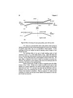
Figure 1.17 Configuration for
Problem 1.12
1.12 What is the temperature at the left-hand wall shown in Fig. 1.17.
Both walls are thin, very large in extent, highly conducting, and
thermally black. [T
right
= 42.5
◦
C.]
1.13 Develop S.I. to English conversion factors for:
• The thermal diffusivity, α
• The heat flux, q
• The density, ρ
• The Stefan-Boltzmann constant, σ
• The view factor, F

1–2
• The molar entropy
• The specific heat per unit mass, c
In each case, begin with basic dimension J, m, kg, s,
◦
C, and
check your answers against Appendix B if possible.
1.14 Three infinite, parallel, black, opaque plates transfer heat by
radiation, as shown in Fig. 1.18. Find T
2
.
1.15 Four infinite, parallel, black, opaque plates transfer heat by
radiation, as shown in Fig. 1.19. Find T
2
and T
3
.[T
2
= 75.53
◦
C.]
1.16 Two large, black, horizontal plates are spaced a distance L
from one another. The top one is warm at a controllable tem-
40 Chapter 1: Introduction
Figure 1.18 Configuration for
Problem 1.14
perature, T
h
, and the bottom one is cool at a specified temper-
ature, T

c
. A gas separates them. The gas is stationary because
it is warm on the top and cold on the bottom. Write the equa-
tion q
rad
/q
cond
= fn(N, Θ ≡ T
h
/T
c
), where N is a dimension-
less group containing σ, k, L, and T
c
. Plot N as a function of
Θ for q
rad
/q
cond
= 1, 0.8, and 1.2 (and for other values if you
wish).
Now suppose that you have a system in which L = 10 cm,
T
c
= 100 K, and the gas is hydrogen with an average k of
0.1 W/m·K . Further suppose that you wish to operate in such a
way that the conduction and radiation heat fluxes are identical.
Identify the operating point on your curve and report the value
of T
h

that you must maintain.
Figure 1.19 Configuration for
Problem 1.15
1.17 A blackened copper sphere 2 cm in diameter and uniformly at
200
◦
C is introduced into an evacuated black chamber that is
maintained at 20
◦
C.
Problems 41
• Write a differential equation that expresses T(t) for the
sphere, assuming lumped thermal capacity.
• Identify a dimensionless group, analogous to the Biot num-
ber, than can be used to tell whether or not the lumped-
capacity solution is valid.
• Show that the lumped-capacity solution is valid.
• Integrate your differential equation and plot the temper-
ature response for the sphere.
1.18 As part of a space experiment, a small instrumentation pack-
age is released from a space vehicle. It can be approximated
as a solid aluminum sphere, 4 cm in diameter. The sphere is
initially at 30
◦
C and it contains a pressurized hydrogen com-
ponent that will condense and malfunction at 30 K. If we take
the surrounding space to be at 0 K, how long may we expect the
implementation package to function properly? Is it legitimate
to use the lumped-capacity method in solving the problem?
(Hint: See the directions for Problem 1.17.) [Time = 5.8 weeks.]

Figure 1.20 Configuration for
Problem 1.19
1.19 Consider heat conduction through the wall as shown in Fig. 1.20.
Calculate q and the temperature of the right-hand side of the
wall.
1.20 Throughout Chapter 1 we have assumed that the steady tem-
perature distribution in a plane uniform wall in linear. To
prove this, simplify the heat diffusion equation to the form
appropriate for steady flow. Then integrate it twice and elimi-
nate the two constants using the known outside temperatures
T
left
and T
right
at x = 0 and x = wall thickness, L.
42 Chapter 1: Introduction
1.21 The thermal conductivity in a particular plane wall depends as
follows on the wall temperature: k = A +BT, where A and B
are constants. The temperatures are T
1
and T
2
on either side
if the wall, and its thickness is L. Develop an expression for q.
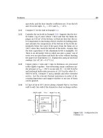
Figure 1.21 Configuration for
Problem 1.22
1.22 Find k for the wall shown in Fig. 1.21. Of what might it be
made?
1.23 What are T
i

, T
j
, and T
r
in the wall shown in Fig. 1.22?[T
j
=
16.44
◦
C.]
Figure 1.22 Configuration for Problem 1.23
Problems 43
1.24 An aluminum can of beer or soda pop is removed from the
refrigerator and set on the table. If
h is 13.5 W/m
2
K, estimate
when the beverage will be at 15
◦
C. Ignore thermal radiation.
State all of your other assumptions.
1.25 One large, black wall at 27
◦
C faces another whose surface is
127
◦
C. The gap between the two walls is evacuated. If the sec-
ond wall is 0.1 m thick and has a thermal conductivity of 17.5
W/m·K, what is its temperature on the back side? (Assume
steady state.)

1.26 A 1 cm diameter, 1% carbon steel sphere, initially at 200
◦
C, is
cooled by natural convection, with air at 20
◦
C. In this case, h is
not independent of temperature. Instead,
h = 3.51(∆T
◦
C)
1/4
W/m
2
K. Plot T
sphere
as a function of t. Verify the lumped-
capacity assumption.
1.27 A 3 cm diameter, black spherical heater is kept at 1100
◦
C. It
radiates through an evacuated annulus to a surrounding spher-
ical shell of Nichrome V. The shell hasa9cminside diameter
and is 0.3 cm thick. It is black on the inside and is held at
25
◦
C on the outside. Find (a) the temperature of the inner wall
of the shell and (b) the heat transfer, Q. (Treat the shell as a
plane wall.)
1.28 The sun radiates 650 W/m
2

on the surface of a particular lake.
At what rate (in mm/hr) would the lake evaporate away if all of
this energy went to evaporating water? Discuss as many other
ways you can think of that this energy can be distributed (h
fg
for water is 2,257,000 J/kg). Do you suppose much of the 650
W/m
2
goes to evaporation?
1.29 It is proposed to make picnic cups, 0.005 m thick, of a new
plastic for which k = k
o
(1 +aT
2
), where T is expressed in
◦
C,
k
o
= 0.15 W/m·K, and a = 10
−4 ◦
C
−2
. We are concerned with
thermal behavior in the extreme case in which T = 100
◦
Cin
the cup and 0
◦
C outside. Plot T against position in the cup

wall and find the heat loss, q.
44 Chapter 1: Introduction
1.30 A disc-shaped wafer of diamond 1 lb is the target of a very high
intensity laser. The disc is 5 mm in diameter and 1 mm deep.
The flat side is pulsed intermittently with 10
10
W/m
2
of energy
for one microsecond. It is then cooled by natural convection
from that same side until the next pulse. If
h = 10 W/m
2
K and
T
∞
=30
◦
C, plot T
disc
as a function of time for pulses that are 50
s apart and 100 s apart. (Note that you must determine the
temperature the disc reaches before it is pulsed each time.)
1.31 A 150 W light bulb is roughly a 0.006 m diameter sphere. Its
steady surface temperature in room air is 90
◦
C, and h on the
outside is 7 W/m
2
K. What fraction of the heat transfer from

the bulb is by radiation directly from the filament through the
glass? (State any additional assumptions.)
1.32 How much entropy does the light bulb in Problem 1.31 pro-
duce?
1.33 Air at 20
◦
C flows over one side of a thin metal sheet (h = 10.6
W/m
2
K). Methanol at 87
◦
C flows over the other side (h = 141
W/m
2
K). The metal functions as an electrical resistance heater,
releasing 1000 W/m
2
. Calculate (a) the heater temperature, (b)
the heat transfer from the methanol to the heater, and (c) the
heat transfer from the heater to the air.
1.34 A black heater is simultaneously cooled by 20
◦
C air (h = 14.6
W/m
2
K) and by radiation to a parallel black wall at 80
◦
C. What
is the temperature of the first wall if it delivers 9000 W/m
2

.
1.35 An 8 oz. can of beer is taken from a 3
◦
C refrigerator and placed
ina25
◦
C room. The 6.3 cm diameter by 9 cm high can is placed
on an insulated surface (
h = 7.3 W/m
2
K). How long will it
take to reach 12
◦
C? Ignore thermal radiation, and discuss your
other assumptions.
1.36 A resistance heater in the form of a thin sheet runs parallel
with 3 cm slabs of cast iron on either side of an evacuated
cavity. The heater, which releases 8000 W/m
2
, and the cast
iron are very nearly black. The outside surfaces of the cast
Problems 45
iron slabs are kept at 10
◦
C. Determine the heater temperature
and the inside slab temperatures.
1.37 A black wall at 1200
◦
C radiates to the left side of a parallel
slab of type 316 stainless steel, 5 mm thick. The right side of

the slab is to be cooled convectively and is not to exceed 0
◦
C.
Suggest a convective process that will achieve this.
1.38 A cooler keeps one side ofa2cmlayer of ice at −10
◦
C. The
other side is exposed to air at 15
◦
C. What is h just on the
edge of melting? Must
h be raised or lowered if melting is to
progress?
1.39 At what minimum temperature does a black heater deliver its
maximum monochromatic emissive power in the visible range?
Compare your result with Fig. 10.2.
1.40 The local heat transfer coefficient during the laminar flow of
fluid over a flat plate of length L is equal to F/x
1/2
, where F is
a function of fluid properties and the flow velocity. How does
h compare with h(x = L)? (x is the distance from the leading
edge of the plate.)
1.41 An object is initially at a temperature above that of its sur-
roundings. We have seen that many kinds of convective pro-
cesses will bring the object into equilibrium with its surround-
ings. Describe the characteristics of a process that will do so
with the least net increase of the entropy of the universe.
1.42 A 250
◦

C cylindrical copper billet, 4 cm in diameter and 8 cm
long, is cooled in air at 25
◦
C. The heat transfer coefficient
is 5 W/m
2
K. Can this be treated as lumped-capacity cooling?
What is the temperature of the billet after 10 minutes?
1.43 The sun’s diameter is 1,392,000 km, and it emits energy as if
it were a black body at 5777 K. Determine the rate at which it
emits energy. Compare this with a value from the literature.
What is the sun’s energy output in a year?
46 Chapter 1: Introduction
Bibliography of Historical and Advanced Texts
We include no specific references for the ideas introduced in Chapter 1
since these may be found in introductory thermodynamics or physics
books. References 1–6 are some texts which have strongly influenced
the field. The rest are relatively advanced texts or handbooks which go
beyond the present textbook.
References
[1.1] J. Fourier. The Analytical Theory of Heat. Dover Publications, Inc.,
New York, 1955.
[1.2] L. M. K. Boelter, V. H. Cherry, H. A. Johnson, and R. C. Martinelli.
Heat Transfer Notes. McGraw-Hill Book Company, New York, 1965.
Originally issued as class notes at the University of California at
Berkeley between 1932 and 1941.
[1.3] M. Jakob. Heat Transfer. John Wiley & Sons, New York, 1949.
[1.4] W. H. McAdams. Heat Transmission. McGraw-Hill Book Company,
New York, 3rd edition, 1954.
[1.5] W. M. Rohsenow and H. Y. Choi. Heat, Mass and Momentum Trans-

fer. Prentice-Hall, Inc., Englewood Cliffs, N.J., 1961.
[1.6] E. R. G. Eckert and R. M. Drake, Jr. Analysis of Heat and Mass
Transfer. Hemisphere Publishing Corp., Washington, D.C., 1987.
[1.7] H. S. Carslaw and J. C. Jaeger. Conduction of Heat in Solids. Ox-
ford University Press, New York, 2nd edition, 1959. Very compre-
henisve, but quite dense.
[1.8] D. Poulikakos. Conduction Heat Transfer. Prentice-Hall, Inc., En-
glewood Cliffs, NJ, 1994. This book’s approach is very accessible.
Good coverage of solidification.
[1.9] V. S. Arpaci. Conduction Heat Transfer. Ginn Press/Pearson Cus-
tom Publishing, Needham Heights, Mass., 1991. Abridgement of
the 1966 edition, omitting numerical analysis.
References 47
[1.10] W. M. Kays and M. E. Crawford. Convective Heat and Mass Trans-
fer. McGraw-Hill Book Company, New York, 3rd edition, 1993.
Coverage is mainly of boundary layers and internal flows.
[1.11] F.M. White. Viscous Fluid Flow. McGraw-Hill, Inc., New York, 2nd
edition, 1991. Excellent development of fundamental results for
boundary layers and internal flows.
[1.12] J.A. Schetz. Foundations of Boundary Layer Theory for Momentum,
Heat, and Mass Transfer. Prentice-Hall, Inc., Englewood Cliffs, NJ,
1984. This book shows many experimental results in support of
the theory.
[1.13] A. Bejan. Convection Heat Transfer. John Wiley & Sons, New York,
2nd edition, 1995. This book makes good use of scaling argu-
ments.
[1.14] M. Kaviany. Principles of Convective Heat Transfer. Springer-
Verlag, New York, 1995. This treatise is wide-ranging and quite
unique. Includes multiphase convection.
[1.15] H. Schlichting and K. Gersten. Boundary-Layer Theory. Springer-

Verlag, Berlin, 8th edition, 2000. Very comprehensive develop-
ment of boundary layer theory. A classic.
[1.16] H. C. Hottel and A. F. Sarofim. Radiative Transfer. McGraw-Hill
Book Company, New York, 1967.
[1.17] R. Siegel and J. R. Howell. Thermal Radiation Heat Transfer. Taylor
and Francis-Hemisphere, Washington, D.C., 4th edition, 2001.
[1.18] M. F. Modest. Radiative Heat Transfer. McGraw-Hill, New York,
1993.
[1.19] P. B. Whalley. Boiling, Condensation, and Gas-Liquid Flow. Oxford
University Press, Oxford, 1987.
[1.20] J. G. Collier and J. R. Thome. Convective Boiling and Condensation.
Oxford University Press, Oxford, 3rd edition, 1994.
[1.21] Y. Y. Hsu and R. W. Graham. Transport Processes in Boiling and
Two-Phase Systems Including Near-Critical Systems. American Nu-
clear Society, LaGrange Park, IL, 1986.
48 Chapter 1: Introduction
[1.22] W. M. Kays and A. L. London. Compact Heat Exchangers. McGraw-
Hill Book Company, New York, 3rd edition, 1984.
[1.23] G. F. Hewitt, editor. Heat Exchanger Design Handbook 1998. Begell
House, New York, 1998.
[1.24] R. B. Bird, W. E. Stewart, and E. N. Lightfoot. Transport Phenomena.
John Wiley & Sons, Inc., New York, 1960.
[1.25] A. F. Mills. Mass Transfer. Prentice-Hall, Inc., Upper Saddle River,
2001. Mass transfer from a mechanical engineer’s perpective with
strong coverage of convective mass transfer.
[1.26] D. S. Wilkinson. Mass Transfer in Solids and Fluids. Cambridge
University Press, Cambridge, 2000. A systematic development of
mass transfer with a materials science focus and an emphasis on
modelling.
[1.27] D. R. Poirier and G. H. Geiger. Transport Phenomena in Materials

Processing. The Minerals, Metals & Materials Society, Warrendale,
Pennsylvania, 1994. A comprehensive introduction to heat, mass,
and momentum transfer from a materials science perspective.
[1.28] W. M. Rohsenow, J. P. Hartnett, and Y. I. Cho, editors. Handbook
of Heat Transfer. McGraw-Hill, New York, 3rd edition, 1998.
2. Heat conduction concepts,
thermal resistance, and the
overall heat transfer coefficient
It is the fire that warms the cold, the cold that moderates the heat the
general coin that purchases all things
Don Quixote, M. de Cervantes, 1615
2.1 The heat diffusion equation
Objective
We must now develop some ideas that will be needed for the design of
heat exchangers. The most important of these is the notion of an overall
heat transfer coefficient. This is a measure of the general resistance of a
heat exchanger to the flow of heat, and usually it must be built up from
analyses of component resistances. In particular, we must know how to
predict
h and how to evaluate the conductive resistance of bodies more
complicated than plane passive walls. The evaluation of
h is a matter
that must be deferred to Chapter 6 and 7. For the present,
h values must
be considered to be given information in any problem.
The heat conduction component of most heat exchanger problems is
more complex than the simple planar analyses done in Chapter 1.To
do such analyses, we must next derive the heat conduction equation and
learn to solve it.
Consider the general temperature distribution in a three-dimensional

body as depicted in Fig. 2.1. For some reason (heating from one side,
in this case), there is a space- and time-dependent temperature field in
the body. This field T = T(x,y,z,t) or T(

r,t), defines instantaneous
49
50 Heat conduction, thermal resistance, and the overall heat transfer coefficient §2.1
Figure 2.1 A three-dimensional, transient temperature field.
isothermal surfaces, T
1
, T
2
, and so on.
We next consider a very important vector associated with the scalar,
T . The vector that has both the magnitude and direction of the maximum
increase of temperature at each point is called the temperature gradient,
∇T :
∇T ≡

i
∂T
∂x
+

j
∂T
∂y
+

k

∂T
∂z
(2.1)
Fourier’s law
“Experience”—that is, physical observation—suggests two things about
the heat flow that results from temperature nonuniformities in a body.
§2.1 The heat diffusion equation 51
These are:

q
|

q|
=−
∇T
|∇T |

This says that

q and ∇T are exactly opposite one
another in direction
and
|

q|∝|∇T|

This says that the magnitude of the heat flux is di-
rectly proportional to the temperature gradient
Notice that the heat flux is now written as a quantity that has a specified
direction as well as a specified magnitude. Fourier’s law summarizes this

physical experience succinctly as

q =−k∇T
(2.2)
which resolves itself into three components:
q
x
=−k
∂T
∂x
q
y
=−k
∂T
∂y
q
z
=−k
∂T
∂z
The coefficient k—the thermal conductivity—also depends on position
and temperature in the most general case:
k = k[

r,T(

r,t)] (2.3)
Fortunately, most materials (though not all of them) are very nearly ho-
mogeneous. Thus we can usually write k = k(T). The assumption that
we really want to make is that k is constant. Whether or not that is legit-

imate must be determined in each case. As is apparent from Fig. 2.2 and
Fig. 2.3, k almost always varies with temperature. It always rises with T
in gases at low pressures, but it may rise or fall in metals or liquids. The
problem is that of assessing whether or not k is approximately constant
in the range of interest. We could safely take k to be a constant for iron
between 0
◦
and 40
◦
C (see Fig. 2.2), but we would incur error between
−100
◦
and 800
◦
C.
It is easy to prove (Problem 2.1) that if k varies linearly with T , and
if heat transfer is plane and steady, then q = k∆T/L, with k evaluated
at the average temperature in the plane. If heat transfer is not planar
or if k is not simply A + BT, it can be much more difficult to specify a
single accurate effective value of k.If∆T is not large, one can still make a
reasonably accurate approximation using a constant average value of k.
Figure 2.2 Variation of thermal conductivity of metallic solids
with temperature
52
Figure 2.3 The temperature dependence of the thermal con-
ductivity of liquids and gases that are either saturated or at 1
atm pressure.
53
54 Heat conduction, thermal resistance, and the overall heat transfer coefficient §2.1
Figure 2.4 Control volume in a

heat-flow field.
Now that we have revisited Fourier’s law in three dimensions, we see
that heat conduction is more complex than it appeared to be in Chapter 1.
We must now write the heat conduction equation in three dimensions.
We begin, as we did in Chapter 1, with the First Law statement, eqn. (1.3):
Q =
dU
dt
(1.3)
This time we apply eqn. (1.3) to a three-dimensional control volume, as
shown in Fig. 2.4.
1
The control volume is a finite region of a conducting
body, which we set aside for analysis. The surface is denoted as S and the
volume and the region as R; both are at rest. An element of the surface,
dS, is identified and two vectors are shown on dS: one is the unit normal
vector,

n (with |

n| = 1), and the other is the heat flux vector,

q =−k∇T ,
at that point on the surface.
We also allow the possibility that a volumetric heat release equal to
˙
q(

r) W/m
3

is distributed through the region. This might be the result of
chemical or nuclear reaction, of electrical resistance heating, of external
radiation into the region or of still other causes.
With reference to Fig. 2.4, we can write the heat conducted out of dS,
in watts, as
(−k∇T)·(

ndS) (2.4)
The heat generated (or consumed) within the region R must be added to
the total heat flow into S to get the overall rate of heat addition to R:
Q =−

S
(−k∇T)·(

ndS) +

R
˙
qdR (2.5)
1
Figure 2.4 is the three-dimensional version of the control volume shown in Fig. 1.8.
§2.1 The heat diffusion equation 55
The rate of energy increase of the region R is
dU
dt
=

R


ρc
∂T
∂t

dR (2.6)
where the derivative of T is in partial form because T is a function of
both

r and t.
Finally, we combine Q, as given by eqn. (2.5), and dU/dt, as given by
eqn. (2.6), into eqn. (1.3). After rearranging the terms, we obtain

S
k∇T ·

ndS =

R

ρc
∂T
∂t
−
˙
q

dR (2.7)
To get the left-hand side into a convenient form, we introduce Gauss’s
theorem, which converts a surface integral into a volume integral. Gauss’s
theorem says that if


A is any continuous function of position, then

S

A ·

ndS =

R
∇·

AdR (2.8)
Therefore, if we identify

A with (k∇T), eqn. (2.7) reduces to

R

∇·k∇T − ρc
∂T
∂t
+
˙
q

dR = 0 (2.9)
Next, since the region R is arbitrary, the integrand must vanish identi-
cally.
2

We therefore get the heat diffusion equation in three dimensions:
∇·k∇T +
˙
q = ρc
∂T
∂t
(2.10)
The limitations on this equation are:
• Incompressible medium. (This was implied when no expansion
work term was included.)
• No convection. (The medium cannot undergo any relative motion.
However, it can be a liquid or gas as long as it sits still.)
2
Consider

f(x)dx =0. Iff(x) were, say, sin x, then this could only be true
over intervals of x = 2π or multiples of it. For eqn. (2.9) to be true for any range of
integration one might choose, the terms in parentheses must be zero everywhere.
56 Heat conduction, thermal resistance, and the overall heat transfer coefficient §2.1
If the variation of k with T is small, k can be factored out of eqn. (2.10)
to get
∇
2
T +
˙
q
k
=
1
α

∂T
∂t
(2.11)
This is a more complete version of the heat conduction equation [recall
eqn. (1.14)] and α is the thermal diffusivity which was discussed after
eqn. (1.14). The term ∇
2
T ≡∇·∇T is called the Laplacian. It arises thus
in a Cartesian coordinate system:
∇·k∇T  k∇·∇T = k


i
∂
∂x
+

j
∂
∂y
+

k
∂
∂x

·


i

∂T
∂x
+

j
∂T
∂y
+

k
∂T
∂z

or
∇
2
T =
∂
2
T
∂x
2
+
∂
2
T
∂y
2
+
∂

2
T
∂z
2
(2.12)
The Laplacian can also be expressed in cylindrical or spherical coor-
dinates. The results are:
• Cylindrical:
∇
2
T ≡
1
r
∂
∂r

r
∂T
∂r

+
1
r
2
∂
2
T
∂θ
2
+

∂
2
T
∂z
2
(2.13)
• Spherical:
∇
2
T ≡
1
r
∂
2
(r T)
∂r
2
+
1
r
2
sin θ
∂
∂θ

sin θ
∂T
∂θ

+

1
r
2
sin
2
θ
∂
2
T
∂φ
2
(2.14a)
or
≡
1
r
2
∂
∂r

r
2
∂T
∂r

+
1
r
2
sin θ

∂
∂θ

sin θ
∂T
∂θ

+
1
r
2
sin
2
θ
∂
2
T
∂φ
2
(2.14b)
where the coordinates are as described in Fig. 2.5.
Figure 2.5 Cylindrical and spherical coordinate schemes.
57
58 Heat conduction, thermal resistance, and the overall heat transfer coefficient §2.2
2.2 Solutions of the heat diffusion equation
We are now in position to calculate the temperature distribution and/or
heat flux in bodies with the help of the heat diffusion equation. In every
case, we first calculate T(

r,t). Then, if we want the heat flux as well, we

differentiate T to get q from Fourier’s law.
The heat diffusion equation is a partial differential equation (p.d.e.)
and the task of solving it may seem difficult, but we can actually do a
lot with fairly elementary mathematical tools. For one thing, in one-
dimensional steady-state situations the heat diffusion equation becomes
an ordinary differential equation (o.d.e.); for another, the equation is lin-
ear and therefore not too formidable, in any case. Our procedure can be
laid out, step by step, with the help of the following example.
Example 2.1 Basic Method
A large, thin concrete slab of thickness L is “setting.” Setting is an
exothermic process that releases
˙
q W/m
3
. The outside surfaces are
kept at the ambient temperature, so T
w
= T
∞
. What is the maximum
internal temperature?
Solution.
Step 1. Pick the coordinate scheme that best fits the problem and iden-
tify the independent variables that determine T. In the example,
T will probably vary only along the thin dimension, which we will
call the x-direction. (We should want to know that the edges are
insulated and that L was much smaller than the width or height.
If they are, this assumption should be quite good.) Since the in-
terior temperature will reach its maximum value when the pro-
cess becomes steady, we write T = T(x only).

Step 2. Write the appropriate d.e., starting with one of the forms of
eqn. (2.11).
∂
2
T
∂x
2
+
∂
2
T
∂y
2
+
∂
2
T
∂z
2
  
=0, since
T ≠ T(y or z)
+
˙
q
k
=
1
α
∂T

∂t

 
= 0, since
steady
Therefore, since T = T(x only), the equation reduces to the
§2.2 Solutions of the heat diffusion equation 59
ordinary d.e.
d
2
T
dx
2
=−
˙
q
k
Step 3. Obtain the general solution of the d.e. (This is usually the
easiest step.) We simply integrate the d.e. twice and get
T =−
˙
q
2k
x
2
+C
1
x +C
2
Step 4. Write the “side conditions” on the d.e.—the initial and bound-

ary conditions. This is always the hardest part for the beginning
students; it is the part that most seriously tests their physical
or “practical” understanding of problems.
Normally, we have to make two specifications of temperature
on each position coordinate and one on the time coordinate to
get rid of the constants of integration in the general solution.
(These matters are discussed at greater length in Chapter 4.)
In this case there are two boundary conditions:
T(x = 0) = T
w
and T(x = L) = T
w
Very Important Warning: Never, never introduce inaccessible
information in a boundary or initial condition. Always stop and
ask yourself, “Would I have access to a numerical value of the
temperature (or other data) that I specify at a given position or
time?” If the answer is no, then your result will be useless.
Step 5. Substitute the general solution in the boundary and initial con-
ditions and solve for the constants. This process gets very com-
plicated in the transient and multidimensional cases. Fourier
series methods are typically needed to solve the problem. How-
ever, the steady one-dimensional problems are usually easy. In
the example, by evaluating at x = 0 and x = L, we get:
T
w
=−0 + 0 +C
2
so C
2
= T

w
T
w
=−
˙
qL
2
2k
+C
1
L + C
2

=T
w
so C
1
=
˙
qL
2k
60 Heat conduction, thermal resistance, and the overall heat transfer coefficient §2.2
Figure 2.6 Temperature distribution in the setting concrete
slab Example 2.1.
Step 6. Put the calculated constants back in the general solution to get
the particular solution to the problem. In the example problem
we obtain:
T =−
˙
q

2k
x
2
+
˙
q
2k
Lx +T
w
This should be put in neat dimensionless form:
T − T
w
˙
qL
2

k
=
1
2

x
L
−

x
L

2


(2.15)
Step 7. Play with the solution—look it over—see what it has to tell you.
Make any checks you can think of to be sure it is correct. In this
case we plot eqn. (2.15) in Fig. 2.6. The resulting temperature
distribution is parabolic and, as we would expect, symmetrical.
It satisfies the boundary conditions at the wall and maximizes
in the center. By nondimensionalizing the result, we have suc-
ceeded in representing all situations with a simple curve. That
is highly desirable when the calculations are not simple, as they
are here. (Notice that T actually depends on five different things,
yet the solution is a single curve on a two-coordinate graph.)
§2.2 Solutions of the heat diffusion equation 61
Finally, we check to see if the heat flux at the wall is correct:
q
wall
=−k
∂T
∂x




x=0
= k

˙
q
k
x −
˙

qL
2k

x=0
=−
˙
qL
2
Thus, half of the total energy generated in the slab comes out
of the front side, as we would expect. The solution appears to
be correct.
Step 8. If the temperature field is now correctly established, you can,
if you wish, calculate the heat flux at any point in the body by
substituting T(

r,t)back into Fourier’s law. We did this already,
in Step 7, to check our solution.
We shall run through additional examples in this section and the fol-
lowing one. In the process, we shall develop some important results for
future use.
Example 2.2 The Simple Slab
A slab shown in Fig. 2.7 is at a steady state with dissimilar temper-
atures on either side and no internal heat generation. We want the
temperature distribution and the heat flux through it.
Solution. These can be found quickly by following the steps set
down in Example 2.1:
Figure 2.7 Heat conduction in a slab (Example 2.2).
62 Heat conduction, thermal resistance, and the overall heat transfer coefficient §2.3
Step 1. T = T(x)for steady x-direction heat flow
Step 2.

d
2
T
dx
2
= 0, the steady 1-D heat equation with no
˙
q
Step 3. T = C
1
x +C
2
is the general solution of that equation
Step 4. T(x = 0) = T
1
and T(x = L) = T
2
are the b.c.s
Step 5. T
1
= 0 + C
2
, so C
2
= T
1
; and T
2
= C
1

L + C
2
, so C
1
=
T
2
−T
1
L
Step 6. T = T
1
+
T
2
−T
1
L
x;or
T − T
1
T
2
−T
1
=
x
L
Step 7. We note that the solution satisfies the boundary conditions
and that the temperature profile is linear.

Step 8. q =−k
dT
dx
=−k
d
dx

T
1
−
T
1
−T
2
L
x

so that
q = k
∆T
L
This result, which is the simplest heat conduction solution, calls to
mind Ohm’s law. Thus, if we rearrange it:
Q =
∆T
L/kA
is like I =
E
R
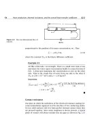
where L/kA assumes the role of a thermal resistance, to which we give

the symbol R
t
. R
t
has the dimensions of (K/W). Figure 2.8 shows how we
can represent heat flow through the slab with a diagram that is perfectly
analogous to an electric circuit.
2.3 Thermal resistance and the electrical analogy
Fourier’s, Fick’s, and Ohm’s laws
Fourier’s law has several extremely important analogies in other kinds of
physical behavior, of which the electrical analogy is only one. These anal-
ogous processes provide us with a good deal of guidance in the solution
of heat transfer problems And, conversely, heat conduction analyses can
often be adapted to describe those processes.
§2.3 Thermal resistance and the electrical analogy 63
Figure 2.8 Ohm’s law analogy to conduction through a slab.
Let us first consider Ohm’s law in three dimensions:
flux of electrical charge =

I
A
≡

J =−γ∇V (2.16)

I amperes is the vectorial electrical current, A is an area normal to the
current vector,

J is the flux of current or current density, γ is the electrical
conductivity in cm/ohm·cm

2
, and V is the voltage.
To apply eqn. (2.16) to a one-dimensional current flow, as pictured in
Fig. 2.9, we write eqn. (2.16)as
J =−γ
dV
dx
= γ
∆V
L
, (2.17)
but ∆V is the applied voltage, E, and the resistance of the wire is R ≡
L

γA. Then, since I = JA, eqn. (2.17) becomes
I =
E
R
(2.18)
which is the familiar, but restrictive, one-dimensional statement of Ohm’s
law.
Fick’s law is another analogous relation. It states that during mass
diffusion, the flux,

j
1
, of a dilute component, 1, into a second fluid, 2, is