A HEAT TRANSFER TEXTBOOK - THIRD EDITION Episode 3 Part 8 pps

664 An introduction to mass transfer §11.9
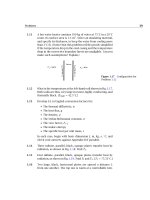
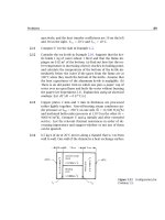
Figure 11.20 The wet bulb of a sling psychrometer.
perature, is directly related to the amount of water in the surrounding
air.
12
The highest ambient air temperatures we normally encounter are fairly
low, so the rate of mass transfer should be small. We can test this sug-
gestion by computing an upper bound on B
m,H
2
O
, under conditions that
should maximize the evaporation rate: using the highest likely air tem-
perature and the lowest humidity. Let us set those values, say, at 120
◦
F
(49
◦
C) and zero humidity (m
H
2
O,e
= 0).
We know that the vapor pressure on the wet bulb will be less than the
saturation pressure at 120
◦
F, since evaporation will keep the bulb at a
lower temperature:
x
H
2

O,s
 p
sat
(120
◦
F)/p
atm
= (11, 671 Pa)/(101, 325 Pa) = 0.115
12
The wet-bulb temperature for air–water systems is very nearly the adiabatic satu-
ration temperature of the air–water mixture — the temperature reached by a mixture
if it is brought to saturation with water by adding water vapor without adding heat. It
is a thermodynamic property of an air–water combination.
§11.9 Simultaneous heat and mass transfer 665
so, with eqn. (11.67),
m
H
2
O,s
 0.0750
Thus, our criterion for low-rate mass transfer, eqn. (11.74), is met:
B
m,H
2
O
=

m
H
2

O,s
−m
H
2
O,e
1 −m
H
2
O,s

 0.0811
Alternatively, in terms of the blowing factor, eqn. (11.104),
ln(1 +B
m,H
2
O
)
B
m,H
2
O
 0.962
This means that under the worst normal circumstances, the low-rate the-
ory should deviate by only 4 percent from the actual rate of evaporation.
We may form an energy balance on the wick by considering the u, s,
and e surfaces shown in Fig. 11.20. At the steady temperature, no heat is
conducted past the u-surface (into the wet bulb), but liquid water flows
through it to the surface of the wick where it evaporates. An energy
balance on the region between the u and s surfaces gives
n

H
2
O,s
ˆ
h
H
2
O,s
  
enthalpy of water
vapor leaving
− q
s
  
heat convected
to the wet bulb
= n
H
2
O,u
ˆ
h
H
2
O,u
  
enthalpy of liquid
water arriving
Since mass is conserved, n
H

2
O,s
= n
H
2
O,u
, and because the enthalpy
change results from vaporization,
ˆ
h
H
2
O,s
−
ˆ
h
H
2
O,u
= h
fg
. Hence,
n
H
2
O,s
h
fg



T
wet-bulb
= h(T
e
−T
wet-bulb
)
For low-rate mass transfer, n
H
2
O,s
 j
H
2
O,s
, and this equation can be
written in terms of the mass transfer coefficient
g
m,H
2
O

m
H
2
O,s
−m
H
2
O,e


h
fg


T
wet-bulb
= h(T
e
−T
wet-bulb
) (11.107)
The heat and mass transfer coefficients depend on the geometry and
flow rates of the psychrometer, so it would appear that T
wet-bulb
should
depend on the device used to measure it. The two coefficients are not in-
dependent, however, owing to the analogy between heat and mass trans-
fer. For forced convection in cross flow, we saw in Chapter 7 that the
heat transfer coefficient had the general form
hD
k
= C Re
a
Pr
b
666 An introduction to mass transfer §11.9
where C is a constant, and typical values of a and b are a  1/2 and
b  1/3. From the analogy,
g

m
D
ρD
12
= C Re
a
Sc
b
Dividing the second expression into the first, we find
h
g
m
c
p
D
12
α
=

Pr
Sc

b
Both α/D
12
and Sc/Pr are equal to the Lewis number, Le. Hence,
h
g
m
c

p
= Le
1−b
 Le
2/3
(11.108)
The Lewis number for air–water systems is about 0.847. Eqn. (11.108)
shows that the ratio of h to g
m
depends primarily on the physical prop-
erties of the mixture, rather than the geometry or flow rate.
This type of relationship between h and g
m
was first developed by
W. K. Lewis in 1922 for the case in which Le = 1[11.27]. (Lewis’s pri-
mary interest was in air–water systems, so the approximation was not
too bad.) The more general form, eqn. (11.108), is another Reynolds-
Colburn type of analogy, similar to eqn. (6.76). It was given by Chilton
and Colburn [11.28] in 1934.
Equation (11.107) may now be written as
T
e
−T
wet-bulb
=

h
fg



T
wet-bulb
c
p
Le
2/3


m
H
2
O,s
−m
H
2
O,e

(11.109)
This expression can be solved iteratively with a steam table to obtain the
wet-bulb temperature as a function of the dry-bulb temperature, T
e
, and
the humidity of the ambient air, m
H
2
O,e
. The psychrometric charts found
in engineering handbooks and thermodynamics texts can be generated in
this way. We ask the reader to make such calculations in Problem 11.49.
The wet-bulb temperature is a helpful concept in many phase-change

processes. When a small body without internal heat sources evaporates
or sublimes, it cools to a steady “wet-bulb” temperature at which con-
vective heating is balanced by latent heat removal. The body will stay at
that temperature until the phase-change process is complete. Thus, the
wet-bulb temperature appears in the evaporation of water droplets, the
sublimation of dry ice, the combustion of fuel sprays, and so on. If the
body is massive, however, steady state may not be reached very quickly.
§11.9 Simultaneous heat and mass transfer 667
Stagnant film model of heat transfer at high mass transfer rates
The multicomponent energy equation. Each species in a mixture car-
ries its own enthalpy,
ˆ
h
i
. In a flow with mass transfer, different species
move with different velocities, so that enthalpy transport by individ-
ual species must enter the energy equation along with heat conduction
through the fluid mixture. For steady, low-speed flow without internal
heat generation or chemical reactions, we may rewrite the energy balance,
eqn. (6.36), as
−

S
(−k∇T)· d

S −

S




i
ρ
i
ˆ
h
i

v
i


·d

S = 0
where the second term accounts for the enthalpy transport by each species
in the mixture. The usual procedure of applying Gauss’s theorem and re-
quiring the integrand to vanish identically gives
∇·


−k∇T +

i
ρ
i
ˆ
h
i


v
i


= 0 (11.110)
This equation shows that the total energy flux—the sum of heat conduc-
tion and enthalpy transport—is conserved in steady flow.
13
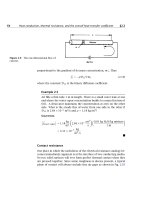
The stagnant film model. Let us restrict attention to the transport of a
single species, i, across a boundary layer. We again use the stagnant film
model for the thermal boundary layer and consider the one-dimensional
flow of energy through it (see Fig. 11.21). Equation (11.110) simplifies to
d
dy

−k
dT
dy
+ρ
i
ˆ
h
i
v
i

= 0 (11.111)
From eqn. (11.69) for steady, one-dimensional mass conservation
n
i

= constant in y = n
i,s
13
The multicomponent energy equation becomes substantially more complex when
kinetic energy, body forces, and thermal or pressure diffusion are taken into account.
The complexities are such that most published derivations of the multicomponent
energy equation are incorrect, as shown by Mills in 1998 [11.29]. The main source
of error has been the assignment of an independent kinetic energy to the ordinary
diffusion velocity. This leads to such inconsistencies as a mechanical work term in the
thermal energy equation.
668 An introduction to mass transfer §11.9
Figure 11.21 Energy transport in a stagnant film.
If we neglect pressure variations and assume a constant specific heat
capacity (as in Sect. 6.3), the enthalpy may be written as
ˆ
h
i
= c
p,i
(T −T
ref
),
and eqn. (11.111) becomes
d
dy

−k
dT
dy
+n

i,s
c
p,i
T

= 0
Integrating twice and applying the boundary conditions
T(y = 0) = T
s
and T(y = δ
t
) = T
e
we obtain the temperature profile of the stagnant film:
T −T
s
T
e
−T
s
=
exp

n
i,s
c
p,i
k
y


−1
exp

n
i,s
c
p,i
k
δ
t

−1
(11.112)
The temperature distribution may be used to find the heat transfer
coefficient according to its definition [eqn. (6.5)]:
h ≡
−k
dT
dy





s
T
s
−T
e
=

n
i,s
c
p,i
exp

n
i,s
c
p,i
k
δ
t

−1
(11.113)
We define the heat transfer coefficient in the limit of zero mass transfer,
h
∗
,as
h
∗
≡ lim
n
i,s
→0
h =
k
δ
t

(11.114)
§11.9 Simultaneous heat and mass transfer 669
Substitution of eqn. (11.114) into eqn. (11.113) yields
h =
n
i,s
c
p,i
exp(n
i,s
c
p,i
/h
∗
) −1
(11.115)
To use this result, one first calculates the heat transfer coefficient as if
there were no mass transfer, using the methods of Chapters 6 through 8.
The value obtained is h
∗
, which is then placed in eqn. (11.115) to de-
termine h in the presence of mass transfer. Note that h
∗
defines the
effective film thickness δ
t
through eqn. (11.114).
Equation (11.115) shows the primary effects of mass transfer on h.
When n
i,s

is large and positive—the blowing case—h becomes smaller
than h
∗
. Thus, blowing decreases the heat transfer coefficient, just as it
decreases the mass transfer coefficient. Likewise, when n
i,s
is large and
negative—the suction case—h becomes very large relative to h
∗
: suc-
tion increases the heat transfer coefficient just as it increases the mass
transfer coefficient.
Condition for the low-rate approximation. When the rate of mass trans-
fer is small, we may approximate h by h
∗
, just as we approximated g
m
by g
∗
m
at low mass transfer rates. The approximation h = h
∗
may be
tested by considering the ratio n
i,s
c
p,i
/h
∗
in eqn. (11.115). For example,

if n
i,s
c
p,i
/h
∗
= 0.2, then h/h
∗
= 0.90, and h = h
∗
within an error of
only 10 percent. This is within the uncertainty to which h
∗
can be pre-
dicted in most flows. In gases, if B
m,i
is small, n
i,s
c
p,i
/h
∗
will usually be
small as well.
Property reference state. In Section 11.8, we calculated g
∗
m,i
(and thus
g
m,i

) at the film temperature and film composition, as though mass
transfer were occurring at the mean mixture composition and tempera-
ture. We may evaluate h
∗
and g
∗
m,i
in the same way when heat and mass
transfer occur simultaneously. If composition variations are not large,
as in many low-rate problems, it may be adequate to use the freestream
composition and film temperature. When large properties variations are
present, other schemes may be required [11.30].
670 An introduction to mass transfer §11.9
Figure 11.22 Transpiration cooling.
Energy balances in simultaneous heat and mass transfer
Transpiration cooling. To calculate simultaneous heat and mass trans-
fer rates, one must generally look at the energy balance below the wall as
well as those at the surface and across the boundary layer. Consider, for
example, the process of transpiration cooling, shown in Fig. 11.22. Here a
wall exposed to high temperature gases is protected by injecting a cooler
gas into the flow through a porous section of the surface. A portion of
the heat transfer to the wall is taken up in raising the temperature of the
transpired gas. Blowing serves to thicken the boundary layer and reduce
h, as well. This process is frequently used to cool turbine blades and
combustion chamber walls.
Let us construct an energy balance for a steady state in which the wall
has reached a temperature T
s
. The enthalpy and heat fluxes are as shown
in Fig. 11.22. We take the coolant reservoir to be far enough back from

the surface that temperature gradients at the r-surface are negligible and
the conductive heat flux, q
r
, is zero. An energy balance between the r -
and u-surfaces gives
n
i,r
ˆ
h
i.r
= n
i,u
ˆ
h
i,u
−q
u
(11.116)
and between the u- and s-surfaces,
n
i,u
ˆ
h
i,u
−q
u
= n
i,s
ˆ
h

i,s
−q
s
(11.117)
§11.9 Simultaneous heat and mass transfer 671
Since there is no change in the enthalpy of the transpired species when
it passes out of the wall,
ˆ
h
i,u
=
ˆ
h
i,s
(11.118)
and, because the process is steady, conservation of mass gives
n
i,r
= n
i,u
= n
i,s
(11.119)
Thus, eqn. (11.117) reduces to
q
s
= q
u
(11.120)
The flux q

u
is the conductive heat flux into the wall, while q
s
is the con-
vective heat transfer from the gas stream,
q
s
= h(T
e
−T
s
) (11.121)
Combining eqns. (11.116) through (11.121), we find
n
i,s

ˆ
h
i,s
−
ˆ
h
i,r

= h(T
e
−T
s
) (11.122)
This equation shows that, at steady state, the heat convection to the

wall is absorbed by the enthalpy rise of the transpired gas. Writing the
enthalpy as
ˆ
h
i
= c
p,i
(T
s
−T
ref
), we obtain
n
i,s
c
p,i
(T
s
−T
r
) = h(T
e
−T
s
) (11.123)
or
T
s
=
hT

e
+n
i,s
c
p,i
T
r
h +n
i,s
c
p,i
(11.124)
It is left as an exercise (Problem 11.47) to show that
T
s
= T
r
+(T
e
−T
r
) exp(−n
i,s
c
p,i
/h
∗
) (11.125)
The wall temperature decreases exponentially to T
r

as the mass flux of
the transpired gas increases. Transpiration cooling may be enhanced by
injecting a gas with a high specific heat.
672 An introduction to mass transfer §11.9
Sweat Cooling. A common variation on transpiration cooling is sweat
cooling, in which a liquid is bled through a porous wall. The liquid is
vaporized by convective heat flow to the wall, and the latent heat of
vaporization acts as a sink. Figure 11.22 also represents this process.
The balances, eqns. (11.116) and (11.117), as well as mass conservation,
eqn. (11.119), still apply, but the enthalpies at the interface now differ by
the latent heat of vaporization:
ˆ
h
i,u
+h
fg
=
ˆ
h
i,s
(11.126)
Thus, eqn. (11.120) becomes
q
s
= q
u
+h
fg
n
i,s

and eqn. (11.122) takes the form
n
i,s

h
fg
+c
p,i
f
(T
s
−T
r
)

= h(T
e
−T
s
) (11.127)
where c
p,i
f
is the specific heat of liquid i. Since the latent heat is generally
much larger than the sensible heat, a comparison of eqn. (11.127)to
eqn. (11.123) exposes the greater efficiency per unit mass flow of sweat
cooling relative to transpiration cooling.
Thermal radiation. When thermal radiation falls on the surface through
which mass is transferred, the additional heat flux must enter the energy
balances. For example, suppose that thermal radiation were present dur-

ing transpiration cooling. Radiant heat flux, q
rad,e
, originating above the
e-surface would be absorbed below the u-surface.
14
Thus, eqn. (11.116)
becomes
n
i,r
ˆ
h
i,r
= n
i,u
ˆ
h
i,u
−q
u
−αq
rad,e
(11.128)
where α is the radiation absorptance. Equation (11.117) is unchanged.
Similarly, thermal radiation emitted by the wall is taken to originate be-
low the u-surface, so eqn. (11.128)isnow
n
i,r
ˆ
h
i,r

= n
i,u
ˆ
h
i,u
−q
u
−αq
rad,e
+q
rad,u
(11.129)
or, in terms of radiosity and irradiation (see Section 10.4)
n
i,r
ˆ
h
i,r
= n
i,u
ˆ
h
i,u
−q
u
−(H − B) (11.130)
for an opaque surface.
14
Remember that the s- and u-surfaces are fictitious elements of the enthalpy bal-
ances at the phase interface. The apparent space between them need be only a few

molecules thick. Thermal radiation therefore passes through the u-surface and is ab-
sorbed below it.
Problems 673
Chemical Reactions. The heat and mass transfer analyses in this sec-
tion and Section 11.8 assume that the transferred species undergo no
homogeneous reactions. If reactions do occur, the mass balances of Sec-
tion 11.8 are invalid, because the mass flux of a reacting species will vary
across the region of reaction. Likewise, the energy balance of this section
will fail because it does not include the heat of reaction.
For heterogeneous reactions, the complications are not so severe. Re-
actions at the boundaries release the heat of reaction released between
the s- and u-surfaces, altering the boundary conditions. The proper sto-
ichiometry of the mole fluxes to and from the surface must be taken into
account, and the heat transfer coefficient [eqn. (11.115)] must be modi-
fied to account for the transfer of more than one species [11.30].
Problems
11.1 Derive: (a) eqns. (11.8); (b) eqns. (11.9).
11.2 A 1000 liter cylinder at 300 K contains a gaseous mixture com-
posed of 0.10 kmol of NH
3
, 0.04 kmol of CO
2
, and 0.06 kmol of
He. (a) Find the mass fraction for each species and the pressure
in the cylinder. (b) After the cylinder is heated to 600 K, what
are the new mole fractions, mass fractions, and molar concen-
trations? (c) The cylinder is now compressed isothermally to a
volume of 600 liters. What are the molar concentrations, mass
fractions, and partial densities? (d) If 0.40 kg of gaseous N
2

is injected into the cylinder while the temperature remains at
600 K, find the mole fractions, mass fractions, and molar con-
centrations. [(a) m
CO
2
= 0.475; (c) c
CO
2
= 0.0667 kmol/m
3
;
(d) x
CO
2
= 0.187.]
11.3 Planetary atmospheres show significant variations of temper-
ature and pressure in the vertical direction. Observations sug-
gest that the atmosphere of Jupiter has the following compo-
sition at the tropopause level:
number density of H
2
= 5.7 ×10
21
(molecules/m
3
)
number density of He = 7.2 × 10
20
(molecules/m
3

)
number density of CH
4
= 6.5 ×10
18
(molecules/m
3
)
number density of NH
3
= 1.3 ×10
18
(molecules/m
3
)
674 Chapter 11: An introduction to mass transfer
Find the mole fraction and partial density of each species at
this level if p = 0.1 atm and T = 113 K. Estimate the num-
ber densities at the level where p = 10 atm and T = 400 K,
deeper within the Jovian troposphere. (Deeper in the Jupiter’s
atmosphere, the pressure may exceed 10
5
atm.)
11.4 Using the definitions of the fluxes, velocities, and concentra-
tions, derive eqn. (11.34) from eqn. (11.27) for binary diffusion.
11.5 Show that D
12
=D
21
in a binary mixture.

11.6 Fill in the details involved in obtaining eqn. (11.31) from eqn.
(11.30).
11.7 Batteries commonly contain an aqueous solution of sulfuric
acid with lead plates as electrodes. Current is generated by
the reaction of the electrolyte with the electrode material. At
the negative electrode, the reaction is
Pb(s) +SO
2−
4
 PbSO
4
(s) +2e
−
where the (s) denotes a solid phase component and the charge
of an electron is −1.609 ×10
−19
coulombs. If the current den-
sity at such an electrode is J = 5 milliamperes/cm
2
, what is
the mole flux of SO
2−
4
to the electrode? (1 amp =1 coulomb/s.)
What is the mass flux of SO
2−
4
? At what mass rate is PbSO
4
produced? If the electrolyte is to remain electrically neutral,

at what rate does H
+
flow toward the electrode? Hydrogen
does not react at the negative electrode. [
˙
m

PbSO
4
= 7.83 ×
10
−5
kg/m
2
·s.]
11.8 The salt concentration in the ocean increases with increasing
depth, z. A model for the concentration distribution in the
upper ocean is
S = 33.25 + 0.75 tanh(0.026z − 3.7)
where S is the salinity in grams of salt per kilogram of ocean
water and z is the distance below the surface in meters. (a) Plot
the mass fraction of salt as a function of z. (The region of rapid
transition of m
salt
(z) is called the halocline.) (b) Ignoring the
effects of waves or currents, compute j
salt
(z). Use a value of
Problems 675
D

salt,water
= 1.5 × 10
−5
cm
2
/s. Indicate the position of maxi-
mum diffusion on your plot of the salt concentration. (c) The
upper region of the ocean is well mixed by wind-driven waves
and turbulence, while the lower region and halocline tend to
be calmer. Using j
salt
(z) from part (b), make a simple estimate
of the amount of salt carried upward in one week ina5km
2
horizontal area of the sea.
11.9 In catalysis, one gaseous species reacts with another on a pas-
sive surface (the catalyst) to form a gaseous product. For ex-
ample, butane reacts with hydrogen on the surface of a nickel
catalyst to form methane and propane. This heterogeneous
reaction, referred to as hydrogenolysis,is
C
4
H
10
+H
2
Ni
→ C
3
H

8
+CH
4
The molar rate of consumption of C
4
H
10
per unit area in the
reaction is
˙
R
C
4
H
10
= A(e
−∆E/R
◦
T
)p
C
4
H
10
p
−2.4
H
2
, where A = 6.3 ×
10

10
kmol/m
2
·s, ∆E = 1.9 × 10
8
J/kmol, and p is in atm.
(a) If p
C
4
H
10
,s
= p
C
3
H
8
,s
= 0.2 atm, p
CH
4
,s
= 0.17 atm, and
p
H
2
,s
= 0.3 atm at a nickel surface with conditions of 440
◦
C

and 0.87 atm total pressure, what is the rate of consumption of
butane? (b) What are the mole fluxes of butane and hydrogen
to the surface? What are the mass fluxes of propane and ethane
away from the surface? (c) What is
˙
m

? What are v, v
∗
, and
v
C
4
H
10
? (d) What is the diffusional mole flux of butane? What
is the diffusional mass flux of propane? What is the flux of Ni?
[(b) n
CH
4
,s
= 0.0441 kg/m
2
·s; (d) j
C
3
H
8
= 0.121 kg/m
2

·s.]
11.10 Consider two chambers held at temperatures T
1
and T
2
, re-
spectively, and joined by a small insulated tube. The chambers
are filled with a binary gas mixture, with the tube open, and
allowed to come to steady state. If the Soret effect is taken
into account, what is the concentration difference between the
two chambers? Assume that an effective mean value of the
thermal diffusion ratio is known.
11.11 Compute D
12
for oxygen gas diffusing through nitrogen gas
at p = 1 atm, using eqns. (11.39) and (11.42), for T = 200 K,
500 K, and 1000 K. Observe that eqn. (11.39) shows large de-
viations from eqn. (11.42), even for such simple and similar
molecules.
676 Chapter 11: An introduction to mass transfer
11.12 (a) Compute the binary diffusivity of each of the noble gases
when they are individually mixed with nitrogen gas at 1 atm
and 300 K. Plot the results as a function of the molecular
weight of the noble gas. What do you conclude? (b) Consider
the addition of a small amount of helium (x
He
= 0.04) to a mix-
ture of nitrogen (x
N
2

= 0.48) and argon (x
Ar
= 0.48). Com-
pute D
He,m
and compare it with D
Ar,m
. Note that the higher
concentration of argon does not improve its ability to diffuse
through the mixture.
11.13 (a) One particular correlation shows that gas phase diffusion
coefficients vary as T
1.81
and p
−1
. If an experimental value of
D
12
is known at T
1
and p
1
, develop an equation to predict D
12
at T
2
and p
2
. (b) The diffusivity of water vapor (1) in air (2) was
measured to be 2.39 ×10

−5
m
2
/sat8
◦
C and 1 atm. Provide a
formula for D
12
(T , p).
11.14 Kinetic arguments lead to the Stefan-Maxwell equation for a
dilute-gas mixture:
∇x
i
=
n

j=1
c
i
c
j
c
2
D
ij



J
∗

j
c
j
−

J
∗
i
c
i


(a) Derive eqn. (11.44) from this, making the appropriate as-
sumptions. (b) Show that if D
ij
has the same value for each
pair of species, then D
im
=D
ij
.
11.15 Compute the diffusivity of methane in air using (a) eqn. (11.42)
and (b) Blanc’s law. For part (b), treat air as a mixture of oxygen
and nitrogen, ignoring argon. Let x
methane
= 0.05, T = 420
◦
F,
and p = 10 psia. [(a) D
CH

4
,air
= 7.66×10
−5
m
2
/s; (b) D
CH
4
,air
=
8.13 ×10
−5
m
2
/s.]
11.16 Diffusion of solutes in liquids is driven by the chemical poten-
tial, µ. Work is required to move a mole of solute A from a
region of low chemical potential to a region of high chemical
potential; that is,
dW = dµ
A
=
dµ
A
dx
dx
under isothermal, isobaric conditions. For an ideal (very dilute)
solute, µ
A

is given by
µ
A
= µ
0
+R
◦
T ln(c
A
)
Problems 677
where µ
0
is a constant. Using an elementary principle of me-
chanics, derive the Nernst-Einstein equation. Note that the so-
lution must be assumed to be very dilute.
11.17 A dilute aqueous solution at 300 K contains potassium ions,
K
+
. If the velocity of aqueous K
+
ions is 6.61 × 10
−4
cm
2
/s·V
per unit electric field (1 V/cm), estimate the effective radius of
K
+
ions in an aqueous solution. Criticize this estimate. (The

charge of an electron is −1.609 × 10
−19
coulomb and a volt =
1J/coulomb.)
11.18 (a) Obtain diffusion coefficients for: (1) dilute CCl
4
diffusing
through liquid methanol at 340 K; (2) dilute benzene diffus-
ing through water at 290 K; (3) dilute ethyl alcohol diffus-
ing through water at 350 K; and (4) dilute acetone diffusing
through methanol at 370 K. (b) Estimate the effective radius of
a methanol molecule in a dilute aqueous solution.
[(a) D
acetone,methanol
= 6.8 ×10
−9
m
2
/s.]
11.19 If possible, calculate values of the viscosity, µ, for methane,
hydrogen sulfide, and nitrous oxide, under the following con-
ditions: 250 K and 1 atm, 500 K and 1 atm, 250 K and 2 atm,
250 K and 12 atm, 500 K and 12 atm.
11.20 (a) Show that k = (5/2)µc
v
for a monatomic gas. (b) Obtain
Eucken’s formula for the Prandtl number of a dilute gas:
Pr = 4γ

(9γ − 5)

(c) Recall that for an ideal gas, γ  (D + 2)/D, where D is the
number of modes of energy storage of its molecules. Obtain
an expression for Pr as a function of D and describe what it
means. (d) Use Eucken’s formula to compute Pr for gaseous
Ar, N
2
, and H
2
O. Compare the result to data in Appendix A
over the range of temperatures. Explain the results obtained
for steam as opposed to Ar and N
2
. (Note that for each mode
of vibration, there are two modes of energy storage but that
vibration is normally inactive until T is very high.)
11.21 A student is studying the combustion of a premixed gaseous
fuel with the following molar composition: 10.3% methane,
15.4% ethane, and 74.3% oxygen. She passes 0.006 ft
3
/softhe
678 Chapter 11: An introduction to mass transfer
mixture (at 70
◦
F and 18 psia) through a smooth 3/8 inch I.D.
tube, 47 inches long. (a) What is the pressure drop? (b) The
student’s advisor recommends preheating the fuel mixture, us-
ing a Nichrome strip heater wrapped around the last 5 inches
of the duct. If the heater produces 0.8W/inch, what is the wall
temperature at the outlet of the duct? Let c
p,CH

4
= 2280 J/kg·K,
γ
CH
4
= 1.3, c
p,C
2
H
6
= 1730 J/kg·K, and γ
C
2
H
6
= 1.2, and evalu-
ate the properties at the inlet conditions.
11.22 (a) Work Problem 6.36. (b) A fluid is said to be incompressible if
the density of a fluid particle does not change as it moves about
in the flow (i.e., if Dρ/Dt = 0). Show that an incompressible
flow satisfies ∇·

u = 0. (c) How does the condition of incom-
pressibility differ from that of “constant density”? Describe a
flow that is incompressible but that does not have “constant
density.”
11.23 Carefully derive eqns. (11.62) and (11.63). Note that ρ is not
assumed constant in eqn. (11.62).
11.24 Derive the equation of species conservation on a molar basis,
using c

i
rather than ρ
i
. Also obtain an equation in c
i
alone,
similar to eqn. (11.63) but without the assumption of incom-
pressibility. What assumptions must be made to obtain the
latter result?
11.25 Find the following concentrations: (a) the mole fraction of air
in solution with water at 5
◦
C and 1 atm, exposed to air at the
same conditions, H = 4.88 × 10
4
atm; (b) the mole fraction
of ammonia in air above an aqueous solution, with x
NH
3
=
0.05 at 0.9 atm and 40
◦
C and H = 1522 mm Hg; (c) the mole
fraction of SO
2
in an aqueous solution at 15
◦
C and 1 atm, if
p
SO

2
= 28.0mmHgandH = 1.42 × 10
4
mm Hg; and (d) the
partial pressure of ethylene over an aqueous solution at 25
◦
C
and 1 atm, with x
C
2
H
4
= 1.75 ×10
−5
and H = 11.4 × 10
3
atm.
11.26 Use a steam table to estimate (a) the mass fraction of water
vapor in air over water at 1 atm and 20
◦
C, 50
◦
C, 70
◦
C, and
90
◦
C; (b) the partial pressure of water over a 3 percent-by-
weight aqueous solution of HCl at 50
◦

C; (c) the boiling point
at 1 atm of salt water with a mass fraction m
NaCl
= 0.18.
[(c) T
B.P.
= 101.8
◦
C.]
Problems 679
11.27 Suppose that a steel fitting with a carbon mass fraction of 0.2%
is put into contact with carburizing gases at 940
◦
C, and that
these gases produce a steady mass fraction of 1.0% carbon at
the surface of the metal. The diffusion coefficient of carbon in
this steel is
D
C,Fe
=

1.50×10
−5
m
2

s

exp


−(1.42 ×10
8
J/kmol)

(R
◦
T)

for T in kelvin. How long does it take to produce a carbon
concentration of 0.6% by mass at a depth of 0.5 mm? How
much less time would it take if the temperature were 980
◦
C?
11.28 (a) Write eqn. (11.62) in its boundary layer form. (b) Write this
concentration boundary layer equation and its b.c.’s in terms
of a nondimensional mass fraction, ψ, analogous to the dimen-
sionless temperature in eqn. (6.42). (c) For ν =D
im
, relate ψ
to the Blasius function, f , for flow over a flat plate. (d) Note the
similar roles of Pr and Sc in the two boundary layer transport
processes. Infer the mass concentration analog of eqn. (6.55)
and sketch the concentration and momentum b.l. profiles for
Sc = 1 and Sc  1.
11.29 When Sc is large, momentum diffuses more easily than mass,
and the concentration b.l. thickness, δ
c
, is much less than the
momentum b.l. thickness, δ. On a flat plate, the small part
of the velocity profile within the concentration b.l. is approxi-

mately u/U
e
= 3y/2δ. Compute Nu
m,x
based on this velocity
profile, assuming a constant wall concentration. (Hint: Use the
mass transfer analogs of eqn. (6.47) and (6.50) and note that
q
w
/ρc
p
becomes j
i,s
/ρ.).
11.30 Consider a one-dimensional, binary gaseous diffusion process
in which species 1 and 2 travel in opposite directions along the
z-axis at equal molar rates. (The gas mixture will be at rest,
with v = 0 if the species have identical molecular weights).
This process is known as equimolar counter-diffusion. (a) What
are the relations between N
1
, N
2
, J
∗
1
, and J
∗
2
? (b) If steady state

prevails and conditions are isothermal and isobaric, what is
the concentration of species 1 as a function of z? (c) Write
the mole flux in terms of the difference in partial pressure of
species 1 between locations z
1
and z
2
.
680 Chapter 11: An introduction to mass transfer
11.31 Consider steady mass diffusion from a small sphere. When
convection is negligible, the mass flux in the radial direction is
n
r,i
= j
r,i
=−ρD
im
dm
i
/dr . If the concentration is m
i,∞
far
from the sphere and m
i,s
at its surface, use a mass balance to
obtain the surface mass flux in terms of the overall concentra-
tion difference (assuming that ρD
im
is constant). Then apply
the definition eqns. (11.94) and (11.78) to show that Nu

m,D
= 2
for this situation.
11.32 An experimental Stefan tube is 1 cm in diameter and 10 cm
from the liquid surface to the top. It is held at 10
◦
C and 8.0 ×
10
4
Pa. Pure argon flows over the top and liquid CCl
4
is at
the bottom. The pool level is maintained while 0.086 ml of
liquid CCl
4
evaporates during a period of 12 hours. What is the
diffusivity of carbon tetrachloride in argon measured under
these conditions? The specific gravity of liquid CCl
4
is 1.59
and its vapor pressure is log
10
p
v
= 8.004−1771/T , where p
v
is expressed in mm Hg and T in K.
11.33 Repeat the analysis given in Section 11.7 on the basis of mass
fluxes, assuming that ρD
im

is constant and neglecting any
buoyancy-driven convection. Obtain the analog of eqn. (11.88).
11.34 In Sections 11.5 and 11.7, it was assumed at points that cD
12
or ρD
12
was independent of position. (a) If the mixture compo-
sition (e.g., x
1
) varies in space, this assumption may be poor.
Using eqn. (11.42) and the definitions from Section 11.2, ex-
amine the composition dependence of these two groups. For
what type of mixture is ρD
12
most sensitive to composition?
What does this indicate about molar versus mass-based analy-
sis? (b) How do each of these groups depend on pressure and
temperature? Is the analysis of Section 11.7 really limited to
isobaric conditions? (c) Do the Prandtl and Schmidt numbers
depend on composition, temperature, or pressure?
11.35 A Stefan tube contains liquid bromine at 320 K and 1.2 atm.
Carbon dioxide flows over the top and is also bubbled up through
the liquid at the rate of 4.4ml/hr. If the distance from the liq-
uid surface to the top is 16 cm and the diameter is 1 cm, what
is the evaporation rate of Br
2
?(p
sat,Br
2
= 0.680 bar at 320 K.)

[N
Br
2
,s
= 1.90 ×10
−6
kmol/m
2
·s.]
11.36 Show that g
m,1
= g
m,2
and B
m,1
= B
m,2
in a binary mixture.
Problems 681
11.37 Demonstrate that stagnant film models of the momentum and
thermal boundary layers reproduce the proper dependence of
C
f,x
and Nu
x
on Re
x
and Pr. Using eqns. (6.31) and (6.55)
to obtain the dependence of δ and δ
t

on Re
x
and Pr, show
that stagnant film models gives eqns. (6.33) and (6.58) within
a constant on the order of unity. [The constants in these re-
sults will differ from the exact results because the effective b.l.
thicknesses of the stagnant film model are not the same as the
exact values—see eqn. (6.57).]
11.38 (a) What is the largest value of the mass transfer driving force
when one species is transferred? What is the smallest value?
(b) Plot the blowing factor as a function of B
m,i
for one species
transferred. Indicate on your graph the regions of blowing,
suction, and low-rate mass transfer. (c) Verify the two limits
used to show that g
∗
m,i
= ρD
im
/δ
c
.
11.39 Nitrous oxide is bled through the surface of a porous 3/8 in.
O.D. tube at 0.025 liter/s per meter of tube length. Air flows
over the tube at 25 ft/s. Both the air and the tube are at 18
◦
C,
and the ambient pressure is 1 atm. Estimate the mean concen-
tration of N

2
O at the tube surface. (Hint: First estimate the
concentration using properties of pure air; then correct the
properties if necessary.)
11.40 Film absorbtion is a process whereby gases are absorbed into
a falling liquid film. Typically, a thin film of liquid runs down
the inside of a vertical tube through which the gas flows. An-
alyze this process under the following assumptions: The film
flow is laminar and of constant thickness, δ
0
, with a velocity
profile given by eqn. (8.48); the gas is only slightly soluble in
the liquid, so that it does not penetrate far beyond the liq-
uid surface and so that liquid properties are unaffected by it;
and, the gas concentration at the s- and u-surfaces (above and
below the liquid-vapor interface, respectively) does not vary
along the length of the tube. The inlet concentration of gas in
the liquid is m
1,0
. Show that the mass transfer is given by
Nu
m,x
=

u
0
x
πD
12


1/2
with u
0
=
(ρ
f
−ρ
g
)gδ
2
0
2µ
f
The mass transfer coefficient here is based on the concentra-
tion difference between the u-surface and the bulk liquid at
682 Chapter 11: An introduction to mass transfer
m
1,0
.(Hint: The small penetration assumption can be used to
reduce the species equation for the film to the diffusion equa-
tion, eqn. 11.72.)
11.41 Benzene vapor flows througha3cmI.D. vertical tube. A thin
film of initially pure water runs down the inside wall of the tube
at a flow rate of 0.3 liter/s. If the tube is 0.5 m long and 40
◦
C,
estimate the rate (in kg/s) at which benzene is absorbed into
water over the entire length of the tube. The mass fraction of
benzene at the u-surface is 0.206. (Hint : Use the result stated
in Problem 11.40. Obtain δ

0
from the results in Chapter 8.)
11.42 A mothball consists of a 2.5 cm diameter sphere of naphtha-
lene (C
10
H
8
) that is hung by a wire in a closet. The solid naph-
thalene slowly sublimates to vapor, which drives off the moths.
The latent heat of sublimation and evaporation rate are low
enough that the wet-bulb temperature is essentially the am-
bient temperature. Estimate the lifetime of this mothball in
a closet with a mean temperature of 20
◦
C. Use the following
data:
σ = 6.18 Å,ε/k
B
= 561.5 K for C
10
H
8
,
and, for solid naphthalene,
ρ
C
10
H
8
= 1145 kg/m

3
at 20
◦
C
The vapor pressure (in mmHg) of solid naphthalene near room
temperature is given approximately by log
10
p
v
= 11.450 −
3729.3/(T K). The integral you obtain can be evaluated nu-
merically.
11.43 In contrast to the napthalene mothball described in Prob. 11.42,
other mothballs are made from paradichlorobenzene (PDB). Es-
timate the lifetime of a 2.5 cm diameter PDB mothball using
the following room temperature property data:
σ = 5.76 Å ε/k
B
= 578.9K M
PDB
= 147.0kg/kmol
log
10

p
v
mmHg

= 11.985 −3570/(T K)
ρ

PDB
= 1248 kg/m
3
Problems 683
11.44 Consider the process of catalysis as described in Problem 11.9.
The mass transfer process involved is the diffusion of the re-
actants to the surface and diffusion of products away from it.
(a) What is
˙
m

in catalysis? (b) Reaction rates in catalysis are
of the form:
˙
R
reactant
= Ae
−∆E/R
◦
T
(p
reactant
)
n
(p
product
)
m
kmol/m
2

·s
for the rate of consumption of a reactant per unit surface
area. The p’s are partial pressures and A, ∆E, n, and m are
constants. Suppose that n = 1 and m = 0 for the reaction
B + C → D. Approximate the reaction rate, in terms of mass,
as
˙
r
B
= A

e
−∆E/R
◦
T
ρ
B,s
kg/m
2
·s
and find the rate of consumption of B in terms of m
B,e
and the
mass transfer coefficient for the geometry in question. (c) The
ratio Da ≡ ρA

e
−∆E/R
◦
T

/g
∗
m
is called the Damkohler number.
Explain its significance in catalysis. What features dominate
the process when Da approaches 0 or ∞? What temperature
range characterizes each?
11.45 One typical kind of mass exchanger is a fixed-bed catalytic re-
actor. A flow chamber of length L is packed with a catalyst
bed. A gas mixture containing some species i to be consumed
by the catalytic reaction flows through the bed at a rate
˙
m. The
effectiveness of such a exchanger (cf. Chapter 3)is
ε = 1 − e
−NTU
, where NTU = g
m,oa
PL/
˙
m
where g
m,oa
is the overall mass transfer coefficient for the cat-
alytic packing, P is the surface area per unit length, and ε is
defined in terms of mass fractions. In testing a 0.5 m catalytic
reactor for the removal of ethane, it is found that the ethane
concentration drops from a mass fraction of 0.36 to 0.05 at a
flow rate of 0.05 kg/s. The packing is known to have a surface
area of 11 m

2
. What is the exchanger effectiveness? What is
the overall mass transfer coefficient in this bed?
11.46 (a) Perform the integration to obtain eqn. (11.112). Then take
the derivative and the limit needed to get eqns. (11.113) and
(11.114). (b) What is the general form of eqn. (11.115) when
more than one species is transferred?
684 Chapter 11: An introduction to mass transfer
11.47 (a) Derive eqn. (11.125) from eqn. (11.124). (b) Suppose that
1.5m
2
of the wing of a spacecraft re-entering the earth’s atmo-
sphere is to be cooled by transpiration; 900 kg of the vehicle’s
weight is allocated for this purpose. The low-rate heat transfer
coefficient is about 1800 W/m
2
·K in the region of interest, and
the hottest portion of re-entry is expected to last 3 minutes. If
the air behind the shock wave ahead of the wing is at 2500
◦
C
and the reservior is at 5
◦
C , which of these gases—H
2
, He, and
N
2
—keeps the surface coolest? (Of course, the result for H
2

is
invalidated by the fact that H
2
would burn under these condi-
tions.)
11.48 Dry ice (solid CO
2
) is used to cool medical supplies transported
by a small plane to a remote village in Alaska. A roughly spher-
ical chunk of dry ice, 5 cm in diameter, falls from the plane
through air at 5
◦
C with a terminal velocity of 15 m/s. If steady
state is reached quickly, what are the temperature and sub-
limation rate of the dry ice? The latent heat of sublimation
is 574 kJ/kg and log
10
(p
v
mmHg) = 9.9082 − 1367.3/(T K).
The temperature will be well below the “sublimation point” of
CO
2
(solid-to-vapor saturation temperature), which is −78.6
◦
C
at 1 atm. Use the heat transfer relation for spheres in a lam-
inar flow,
Nu
D

= 2 + 0.3Re
0.6
D
Pr
1/3
.(Hint: first estimate the
surface temperature using properties for pure air; then correct
the properties if necessary.)
11.49 The following data were taken at a weather station over a pe-
riod of several months:
Date T
dry-bulb
T
wet-bulb
3/15 15.5
◦
C 11.0
◦
C
4/21 22.0 16.8
5/13 27.3 25.8
5/31 32.7 20.0
7/4 39.0 31.2
Use eqn. (11.109) to find the mass fraction of water in the air
at each date. Compare these values to values obtained using a
psychrometric chart.
11.50 Biff Harwell has taken Deb sailing. Deb, and Biff’s towel, fall
into the harbor. Biff rescues them both from a passing dolphin
References 685
and then spreads his wet towel out to dry on the fiberglas fore-

deck of the boat. The incident solar radiation is 1050 W/m
2
;
the ambient air is at 31
◦
C, with m
H
2
O
= 0.017; the wind speed
is 8 knots relative to the boat (1 knot = 1.151 mph); ε
towel

α
towel
 1; and the sky has the properties of a black body at
280 K. The towel is 3 ft long in the windward direction and 2 ft
wide. Help Biff figure out how rapidly (in kg/s) water evapo-
rates from the towel.
11.51 Steam condenses on a 25 cm high, cold vertical wall in a low-
pressure condenser unit. The wall is isothermal at 25
◦
C, and
the ambient pressure is 8000 Pa. Air has leaked into the unit
and has reached a mass fraction of 0.04. The steam–air mix-
ture is at 45
◦
C and is blown downward past the wall at 8 m/s.
(a) Estimate the rate of condensation on the wall. (Hint: The
surface of the condensate film is not at the mixture or wall tem-

perature.) (b) Compare the result of part (a) to condensation
without air in the steam. What do you conclude?
11.52 As part of a coating process, a thin film of ethanol is wiped
onto a thick flat plate, 0.1 m by 0.1 m. The initial thickness
of the liquid film is 0.1 mm, and the initial temperature of
both the plate and the film is 303 K. The air above the film
moves at 10 m/s and has a temperature of 303 K. (a) Assume
that the plate is a poor conductor, so that heat loss into it
can be neglected. After a short initial transient, the liquid
film reaches a steady temperature. Find this temperature and
calculate the time required for the film to evaporate. (b) Dis-
cuss what happens when the plate is a very good conductor
of heat, and estimate the shortest time required for evapora-
tion. Properties of ethanol are as follow: log
10
(p
v
mmHg) =
9.4432 − 2287.8/(T K); h
fg
= 9.3 × 10
5
J/kg; liquid density,
ρ
eth
= 789 kg/m
3
; Sc = 1.30 for ethanol vapor in air; vapor
specific heat capacity, c
p

eth
= 1420 J/kg·K.
References
[11.1] W. C. Reynolds. Energy, from Nature to Man. McGraw-Hill Book
Company, New York, 1974.
686 Chapter 11: An introduction to mass transfer
[11.2] S. Chapman and T. G. Cowling. The Mathematical Theory of
Nonuniform Gases. Cambridge University Press, New York, 2nd
edition, 1964.
[11.3] R. K. Ghai, H. Ertl, and F. A. L. Dullien. Liquid diffusion of non-
electrolytes: Part 1. AIChE J., 19(5):881–900, 1973.
[11.4] R. C. Reid, J. M. Prausnitz, and B. E. Poling. The Properties of Gases
and Liquids. McGraw-Hill Book Company, New York, 4th edition,
1987.
[11.5] P. W. Atkins. Physical Chemistry. W. H. Freeman and Co., New
York, 3rd edition, 1986.
[11.6] D. R. Poirier and G. H. Geiger. Transport Phenomena in Materials
Processing. The Minerals, Metals & Materials Society, Warrendale,
Pennsylvania, 1994.
[11.7] T. R. Marrero and E. A. Mason. Gaseous diffusion coefficients.
J. Phys. Chem. Ref. Data, 1:3–118, 1972.
[11.8] J. O. Hirschfelder, C. F. Curtiss, and R. B. Bird. Molecular Theory
of Gases and Liquids. John Wiley & Sons, Inc., New York, 1964.
[11.9] C. L. Tien and J. H. Lienhard. Statistical Thermodynamics. Hemi-
sphere Publishing Corp., Washington, D.C., rev. edition, 1978.
[11.10] R. A. Svehla. Estimated viscosities and thermal conductivities of
gases at high temperatures. NASA TR R-132, 1962. (Nat. Tech.
Inf. Svcs. N63-22862).
[11.11] C. R. Wilke and C. Y. Lee. Estimation of diffusion coefficients for
gases and vapors. Ind. Engr. Chem., 47:1253, 1955.

[11.12] J. O. Hirschfelder, R. B. Bird, and E. L. Spotz. The transport prop-
erties for non-polar gases. J. Chem. Phys., 16(10):968–981, 1948.
[11.13] J. Millat, J. H. Dymond, and C. A. Nieto de Castro. Transport
Properties of Fluids: Their Correlation, Prediction and Estimation.
Cambridge University Press, Cambridge, UK, 1996.
[11.14] G. E. Childs and H. J. M. Hanley. Applicability of dilute gas trans-
port property tables to real gases. Cryogenics, 8:94–97, 1968.
References 687
[11.15] C. Cercignani. Rarefied Gas Dynamics. Cambridge University
Press, Cambridge, UK, 2000.
[11.16] A. Einstein. Investigations of the Theory Brownian Movement.
Dover Publications, Inc., New York, 1956. (This book is a col-
lection of Einstein’s original papers on the subject, which were
published between 1905 and 1908.).
[11.17] W. Sutherland. A dynamical theory of diffusion for non-
electrolytes and the molecular mass of albumin. Phil. Mag., Ser.
6, 9(54):781–785, 1905.
[11.18] H. Lamb. Hydrodynamics. Dover Publications, Inc., New York,
6th edition, 1945.
[11.19] J. C. M. Li and P. Chang. Self-diffusion coefficient and viscosity in
liquids. J. Chem. Phys., 23(3):518–520, 1955.
[11.20] S. Glasstone, K. J. Laidler, and H. Eyring. The Theory of Rate
Processes. McGraw-Hill Book Company, New York, 1941.
[11.21] C. J. King, L. Hsueh, and K-W. Mao. Liquid phase diffusion of
nonelectrolytes at high dilution. J. Chem. Engr. Data, 10(4):348–
350, 1965.
[11.22] C. R. Wilke. A viscosity equation for gas mixtures. J. Chem. Phys.,
18(4):517–519, 1950.
[11.23] E. A. Mason and S. C. Saxena. Approximate formula for the ther-
mal conductivity of gas mixtures. Phys. Fluids, 1(5):361–369,

1958.
[11.24] J. M. Prausnitz, R. N. Lichtenthaler, and E. G. de Azevedo. Molecu-
lar Thermodynamics of Fluid-Phase Equilibria. Prentice-Hall, En-
glewood Cliffs, N.J., 2nd edition, 1986.
[11.25] R. C. Weast, editor. Handbook of Chemistry and Physics. Chemical
Rubber Co., Cleveland, Ohio, 56th edition, 1976.
[11.26] D. S. Wilkinson. Mass Transfer in Solids and Fluids. Cambridge
University Press, Cambridge, 2000.
[11.27] W. K. Lewis. The evaporation of a liquid into a gas. Mech. Engr.,
44(7):445–446, 1922.
688 Chapter 11: An introduction to mass transfer
[11.28] T. H. Chilton and A. P. Colburn. Mass transfer (absorption) coef-
ficients: Prediction from data on heat transfer and fluid friction.
Ind. Eng. Chem., 26:1183–1187, 1934.
[11.29] A. F. Mills. The use of the diffusion velocity in conservation equa-
tions for multicomponent gas mixtures. Int. J. Heat. Mass Trans-
fer, 41(13):1955–1968, 1998.
[11.30] A. F. Mills. Mass Transfer. Prentice-Hall, Inc., Upper Saddle River,
2001.