Báo cáo lâm nghiệp: "Plant community variability within potential natural vegetation units: a case study from the Bohemian Karst" docx
Bạn đang xem bản rút gọn của tài liệu. Xem và tải ngay bản đầy đủ của tài liệu tại đây (595.59 KB, 17 trang )
JOURNAL OF FOREST SCIENCE, 55, 2009 (11): 485–501
Plant community variability within potential natural
vegetation units: a case study from the Bohemian Karst
P. Šamonil, K. Polesná, P. Unar
Silva Tarouca Research Institute for Landscape and Ornamental Gardening,
Department of Forest Ecology, Brno, Czech Republic
ABSTRACT: Based on a map of potential natural vegetation (PNV), actual vegetation was studied in the Mramor
locality (106.4 ha). A total of 188 relevés were examined using stratified random sampling. A comparison was made
between trends in vegetation variability throughout the entire locality and variability within the defined PNV units.
The stratification of the locality according to PNV units was only partly representative of the main trends in vegetation
variability, especially at ecologically distinctive sites. On the other hand, in areas with a relatively limited ecological
gradient, the sites were “oversampled”. The variability of plant communities within PNV units was high. The results of
this case study suggest that the need for delineation of PNV units which are homogeneous in terms of production, site
and phytocoenosis is overestimated. This delineation neither corresponds to the characteristics of actual ecosystems
nor is necessary for the application of a PNV system. A more suitable unit for the development of such a system would
be, for example, forest type series.
Keywords: vegetation classification; vegetation variability; potential natural vegetation; oak forest; Bohemian Karst
Formalized sampling approaches
The subjective selection of phytocoenological
plots, which were traditionally used for many decades, is being replaced by a formalized selection
process. The main reasons for this change were the
requirement of a representative set of samples from
surveyed territories and the desire to eliminate tautological statements of evidence (e.g. Chytrý 2000).
One of the methods widely used in this formalized
approach to data collection is stratified random
sampling (e.g. Hirzel, Guisan 2002). Unlike entirely random sampling, stratified random sampling
enables the more effective placement of plots along
important gradients of variability and in general
provides more information about vegetation rarity
and diversity (Hessburg et al. 2000). However, this
type of selection requires more detailed data on
the studied territory. In studies of phytocoenosis,
stratified random sampling is applied primarily on
the coarse landscape level (e.g. Cooper, Loftus
1998; Cawsey et al. 2002; Hurst, Allen 2007). In
such cases, the landscape is stratified in advance,
e.g. according to climatic characteristics, geological
bedrock, altitude, or the classification of aerial photographs. Random sampling is subsequently applied
in territorial segments within a specific category. The
choice of underlayers for stratification at fine spatial
levels (tens to hundreds of hectares) is problematic,
as commonly used underlayers are too coarse (e.g.
geological maps at a scale of 1:25,000–1:50,000) and
better data sources are not generally available. There
arises a question whether the forest map of potential
natural vegetation (PNV) would be applicable for
this purpose. In the Czech Republic, such a map is
available at a scale of 1:10,000 (and even 1:5,000 in
Supported by the Ministry of the Environment of the Czech Republic, Projects No. MSM 6293359101 and
VaV SP/2d2/138/08.
J. FOR. SCI., 55, 2009 (11): 485–501
485
national nature reserves) for all forest stands in the
country (Anonymous 1971/1976). Other countries
could make use of similarly constructed systems for
the purposes of stratification (e.g. Pojar et al. 1987;
Pyatt et al. 2001; Schwarz 2005).
The potential natural vegetation map
Research into PNV is currently paid considerable
attention (e.g. Chytrý 1998; Neuhäuslová et al.
1998; Zerbe 1998; Buček, Lacina 2002; Ricotta
et al. 2002; Bohn et al. 2003). PNV maps are a part
of the groundwork for future landscape use planning
(e.g. Zelenková 2000) as well as for assessments
of the stability and naturalness of contemporary
ecosystems (Petříček, Míchal 1999). PNV maps
exist for all forest stands in the Czech Republic,
and were constructed using a Typological System
developed by the Forest Management Institute
(TSFMI) (Anonymous 1971/1976 – further extended by Plíva (1991), Mikeska and Kusbach
(1999), Průša (2001), Viewegh et al. (2003)). This
TSFMI was primarily created for the applied function of landscape classification to be used in future
resource planning. While other systems of PNV
classification exist (e.g. Neuhäuslová et al. 1998),
this study uses the concept of “forest type” (FT) (e.g.
Zlatník 1956; Viewegh 1997). The concept behind
this classification was defined for the “Central European space”, and it assumes that we can distinguish
between types of potential natural vegetation – in this
case forest types (FT) – based on the differentiation
of “permanent” ecological site conditions. This idea
is similar to the theory of PNV by Tüxen (1956) (see
Kowarik 1987; Zerbe 1998; Chytrý 1998), according to which such vegetation that would be the most
competitive for given site conditions is “interpreted”
into the landscape. The factors of time and succession
are eliminated (cf. Stumpel, Kalkhoven 1978). In
the TSFMI classification, FT is a mapping unit of
PNV. Unlike other systems that map potential natural
vegetation, this system requires uniformity of soil,
production and phytocoenosis within a mapping
unit. Therefore, a difference in soils, production or
phytocoenosis at a specific landscape segment calls
for new FT. Subsequently, FTs are aggregated into
superstructural units according to their ecological
affinity. During this stage, the search for ecological
factors which lead to differences in the vegetation
composition is of key importance for general modelling of the structure and development of plant communities (e.g. Austin 2002; Ricotta et al. 2002).
As the future development of the structure of
plant communities is not known, units of the PNV
486
represent selected units of existing vegetation (usually, the vegetation least affected by humans and
most stable in time). There are only a few possible
methods to verify the correctness of the PNV concept (Zerbe 1998), but the theoretical assumption
of the homogeneity of forest types can be verified
by analyzing the variability of actual (namely nearnatural) vegetation.
Our objectives in this study are:
– To assess whether the Czech PNV map is useful as
groundwork for the stratification of the territory
in studying actual vegetation.
– To test whether the variability of actual vegetation
contradicts the concept of PNV according to the
TSFMI.
– To check whether the FTs delineated in the PNV
map are homogeneous in terms of phytocoenosis.
MATERIALS AND METHODS
Area descriptions
The Bohemian Karst is a geomorphic part of the
Brdy Region (Demek et al. 2006). Mean annual total
precipitation is about 500 mm; mean annual temperature is 8–9°C (Tolasz et al. 2007; www.chmu.
cz/). There are significant differences between day
and night temperatures during the growing season,
with maximums of 40°C at a ground level on southern slopes.
The studied area (Mramor) covers 106.4 ha and is
situated in the southern part of the Bohemian Karst
(Fig. 1). The highest elevations in the territory are
the summits of Mramor (472 m a.s.l.) and Šamor
(481 m a.s.l.), while the lowest elevations are at an
altitude of about 350 m a.s.l. The territory is geologically homogeneous, with bedrock built of Devonian
limestones. Ecological conditions vary considerably
km
Fig. 1. Study area: The Bohemian Karst Protected Landscape
Area (in grey) with the studied Mramor locality
J. FOR. SCI., 55, 2009 (11): 485–501
m
Fig. 2. The map of potential natural vegetation in the Mramor
locality (Zelenková 2000). Forest types (in alphabetic order):
1A9 – Aceri-Carpineto-Quercetum lapidosum on limestones,
1C2 – Carpineto-Quercetum subxerothermicum with Poa
nemoralis, 1W2 – (Fagi-) Carpineto-Quercetum calcarium,
1X2 – Corneto-Quercetum (xerothermicum) on Rendzic Leptosols, 1X8 – Corneto-Quercetum (xerothermicum) on Lithic
Leptosols (Rendzic), 2A8 – Aceri-Fageto-Quercetum lapidosum on warm slopes, 2A9 – Aceri-Fageto-Quercetum lapidosum on shady slopes, 2B9 – Fageto-Quercetum mesotrophicum
with Alliaria petiolata, 2C8 – Fageto-Quercetum subxerothermicum on limestones with Brychypodium pinnatum,
2D7 – Fageto-Quercetum acerosum deluvium on limestones,
2H5 – Fageto-Quercetum illimerosum mesotrophicum with
Luzula luzuloides and Carex montana, 2I4 – Fageto-Quercetum illimerosum acidophilum with Melampyrum pratense,
2W1 – Fageto-Quercetum calcarium with Mercurialis perennis, 2W3 – Fageto-Quercetum calcarium with Galium odoratum. The territory is crossed by three roadways
throughout the study area, resulting in a wide range
of habitats, from diluvial sites on northern slopes to
exposed southern slopes with shallow soils. Soils can
be classified as Lithic Leptosols (Rendzic), Rendzic
Leptosols (Humic and Eutric), Chromic Cambisols
and Chromic Luvisols (ISSS-ISRIC-FAO 1998;
Driessen et al. 2001; Michéli et al. 2006). The study
area is within Conservation Zone 1 of the Bohemian
Karst Protected Landscape Area, and the dominant
plant communities are subjected to limited human
impact. The map of PNV for the area is shown in
Fig. 2 (Zelenková 2000). We assume that the quality of PNV mapping achieved in the model territory
is at a similar level as in the remaining area of the
Czech Republic.
There are historical records of the tree composition in the area. In 1645, forests surrounding the
village of Liteň (1 km from the Mramor study site)
were described as being composed predominantly
of oak, and other historical sources also mention
beech, hornbeam and pine (Nožička 1957; Novák,
J. FOR. SCI., 55, 2009 (11): 485–501
Tlapák 1974). A similar tree species composition
was described in both 1711 and 1808; Nožička
(1957) and Novák and Tlapák (1974) reported
a low proportion of aspen and fir in the following
years. In spite of the fact that during the subsequent
150 years, deciduous lowland coppiced (low) forests throughout the Czech Republic were routinely
changed to high forests with a large amount of spruce
and Scotch pine, the Mramor site was still depicted
as coppiced forest on stand maps from 1902. At
present, the Mramor forests are dominated by
Quercus petraea agg., Tilia cordata, Fagus sylvatica
and Carpinus betulus, with mixed – sexual and/or
asexual – origin. The occurrence of allochthonous
tree species (Robinia pseudacacia, Aesculus hippocastanum, Larix decidua, Picea abies, Quercus
cerris) is minimal.
Field sampling
Plots for relevés were selected by formalized manner with the use of stratified random sampling (e.g.
Hirzel, Guisan 2002). In the first step, the Mramor
territory was divided into seven site types (ST),
which we obtained by merging the forest types (Zelenková 2000) according to their ecological affinity. Site types were usually identical with individual
edaphic categories of the PNV system, but we made
exceptions in well-founded cases (e.g. it is difficult
to separate FTs 2B9, 2W1, 2W3 in karst regions
– Šamonil 2005, 2007a,b; Šamonil, Viewegh
2005). These ST types were established specifically
for this study and are not a part of the PNV system.
Some specific forest types (1X2, 1X8, and 2I4; see
Fig. 2) were not merged due to their exceptional
character. Thus, the site type in these cases was
identical to that defined by forest type. Defined forest
types were then subjected to random sampling. The
entire Mramor territory was covered by a graticule
with 25 × 25 m2, which were then selected at random
to determine relevés. The affiliation of the square
centre was decisive in determining the square allocation to a specific ST. If the selected square was
in an environment that was significantly anthropogenically modified (e.g. roadside landing, old road), it
was replaced by the next chosen square. In site types
that were larger than 5% of the total territory area, a
total of 32 squares were selected; for other site types
20 squares were selected (Fig. 3).
Phytocoenological plots of 20 × 20 m were delineated in the field, using navigation by a Garmin
GPS with an approximate positioning error of 5 m.
Vegetation was recorded according to the 11-member classification of abundance and dominance by
487
m
Zlatník (1953) – a modified Braun-Blanquet classification. Vertical stratification according to Zlatník (1975) was used. A total number of 188 relevés
were created in June and July, 2005 and 2006. Only
vascular plant taxa were recorded; mosses and lichens were not assessed. The nomenclature followed
Kubát et al. (2002).
Data analysis
Relevés were recorded in the Turboveg for Windows 2.07 a database programme (Hennekens,
Schaminée 2001). For subsequent analyses, the tree
species layers were merged based on their random
overlapping; e.g. the sum of two layers was calculated
as cs = cx + (100 – cx) × cy, where cs is the resulting
overall cover, and cx and cy are taxon covers in layers
x and y expressed in percent (Tichý, Jason 2006).
In order to study vegetation variability, the entire
set of 188 relevés was classified by means of the hierarchic divisive classification TWINSPAN (Hill 1979)
(Table 1). Analysis was performed with four levels of
the set division. Quantitative characteristics of the
occurrence of plant taxa were taken into consideration by adjusting 3 pseudospecies with the limiting
values of cover at 0, 5 and 25%. This resulted in the
division of the set of relevés into 12 groups, for which
fidelity and constancy of plant taxa were calculated.
Taxon fidelity, i.e. the concentration of species occurrence in vegetation units, was measured using the
phi coefficient (Sokal, Rohlf 1995; Chytrý et al.
2002). The phi coefficient (Φ) of association between
species and units is a statistical measure of the association between two categories. This phi coefficient
was calculated according to the formula
Φ = (N × np – n × Np)/√{n × Np × (N – n) × (N – Np)}
488
Fig. 3. Site types created through the
merging of forest types according to their
ecological affinity: A (Forest Types 1A9,
2A8, 2A9), B (2B9, 2W1, 2W3), C (1W2,
1C2, 2C8), D (2D7, 2H5), E (2I4), F (1X2),
G (1X8). The territory was covered by a
grid at a grain of 25 × 25 m. According
to site types, squares were generated
by random selection for the creation of
relevés (marked with a dot). The territory
is divided by three roadways
where:
N – number of relevés in the data set,
Np – number of relevés in the target unit (in this case the
TWINSPAN category),
n – number of occurrences of the species in the data set,
np – number of occurrences of the species in the target unit.
Calculated phi coefficient values range from –1 to
1, but are then multiplied by 100. The highest phi
value of 1 (recalculated to 100) is achieved if the
species occurs in all relevés of the unit and is absent
elsewhere. Calculations were performed and the
resulting tables produced in Juice 6.4.55 software
(Tichý 2002).
Next, vegetation variability was studied within
the defined site types and in the PNV units. The
constancy and fidelity of plant taxa were calculated
according to the site types (Table 2), identically to
the calculation of vegetation characteristics among
TWINSPAN categories. The classification of relevés
according to the PNV system was then compared
with categorization according to TWINSPAN using
a contingency table. At the same time, we evaluated
how the species composition of individual relevés
agrees with their classification according to the PNV
system using the Frequency-Positive Fidelity Index
(FPFI) (Tichý, Jason 2006). In some cases, the frequency and/or fidelity of plant species indicated a
possible reclassification of the relevé to another PNV
unit (forest type). We also calculated the successfulness of the PNV classification; user’s accuracy and
producer’s accuracy (e.g. Congalton 1991; Nilsson 1998; see also Černá, Chytrý 2005 – sensitivity and positive predictive power) were evaluated
for individual forest types.
Detrended correspondence analysis (DCA) was
used in order to compare vegetation variability
within the entire study area with vegetation variJ. FOR. SCI., 55, 2009 (11): 485–501
Table 1. The synoptic table of 188 relevés from Mramor that were classified by means of the TWINSPAN numerical
classification system into 12 classes (Roman numerals). Data for individual taxa are presented in AB form, where A is
the taxon constancy – frequency of occurrence (%), index B represents the taxon fidelity (see Materials and Methods).
Taxa are arranged by fidelity, classes are arranged by floristic similarity. Values accentuated in the table are fidelity values
over 20 (light grey) and higher than 40 (dark grey). Only those taxa whose fidelity to at least one of the TWINSPAN
categories is ≥ 10 are shown
TWINSPAN divisions
--------------------------------------------------------------------
---||||||||||||||||||||||||||||||||||||||||||||||||||||||||||||||||||||||||||
----||||||||||------------------------------------|||||||||||||||||||||||||||||||||||||
----||||||||||
------------------|||||||||||||||||||||----------------|||||||||||||||||
---------------|||||||||
---------|||||||||---------|||||||||---------||||||||||-------|||||||||
Number of TWINSPAN
category
I
II
III
IV
V
VI
VII
VIII
IX
X
XI
XII
Taxon/Number of relevés
3
4
2
1
3
23
20
36
80
11
3
2
Carduus nutans
67
80.4
.
---
.
---
.
---
.
---
.
---
.
---
.
---
.
---
.
---
.
---
.
---
Echium vulgare
67
80.4
.
---
.
---
.
---
.
---
.
---
.
---
.
---
.
---
.
---
.
---
.
---
Scabiosa ochroleuca
100 79.8
.
---
50
---
.
---
.
---
.
---
.
---
.
---
.
---
.
---
.
---
.
---
Campanula rotundifolia
67
67.0
25
---
.
---
.
---
.
---
.
---
.
---
.
---
.
---
.
---
.
---
.
---
Plantago media ssp. longifolia 67
67.0
25
---
.
---
.
---
.
---
.
---
.
---
.
---
.
---
.
---
.
---
.
---
Dianthus carthusianorum
100 62.8 25
---
.
---
100
---
.
---
.
---
.
---
.
---
.
---
.
---
.
---
.
---
Trifolium arvense
67
58.0
---
50
---
Sanguisorba minor
100 54.2 25
---
50
---
Prunus avium
33
---
100 45.4 100
---
Fraxinus excelsior
33
---
100 45.1 100
---
Poa angustifolia
100
---
100 41.0 50
Prunus spinosa
67
---
Galium glaucum
100
---
Agrimonia eupatoria
33
---
Hypericum perforatum
100
---
Melica transsilvanica
.
---
Vincetoxicum hirundinaria
.
Anthericum ramosum
---
.
---
.
---
.
---
.
---
.
---
.
---
.
---
.
---
---
.
---
9
---
.
---
.
---
.
---
.
---
.
---
.
---
---
.
---
9
---
20
---
11
---
9
---
18
---
67
---
.
---
100
---
.
---
.
---
.
---
17
---
2
---
18
---
.
---
.
---
---
100
---
.
---
17
---
45
6.3
8
---
.
---
.
---
.
---
.
---
100 39.4 100
---
100
---
33
---
26
---
5
---
3
---
.
---
9
---
.
---
.
---
100 39.4 100
---
100
---
.
---
35
---
.
---
8
---
.
---
.
---
.
---
.
---
39.2
50
---
100
---
.
---
.
---
.
---
.
---
.
---
.
---
.
---
.
---
100 33.8 100
---
100
---
67
---
39
---
.
---
25
---
1
---
.
---
.
---
.
---
.
---
.
---
.
---
67
77.6
4
---
.
---
.
---
.
---
.
---
.
---
.
---
---
.
---
.
---
.
---
.
---
57
69.3
.
---
3
---
4
---
.
---
.
---
.
---
.
---
.
---
.
---
.
---
33
---
83
69.1
5
---
8
---
2
---
.
---
.
---
.
---
Betonica officinalis
.
---
.
---
.
---
.
---
.
---
70
68.0
10
---
8
---
.
---
9
---
.
---
.
---
Bupleurum falcatum
.
---
.
---
.
---
.
---
67
---
83
54.6
30
---
14
---
.
---
.
---
.
---
.
---
Hierochloe australis
.
---
.
---
.
---
.
---
.
---
43
54.1
15
---
.
---
.
---
.
---
.
---
.
---
Polygonatum odoratum
.
---
.
---
.
---
.
---
33
---
70
51.6
25
---
11
---
4
---
9
---
.
---
.
---
Cotoneaster integerrimus
.
---
.
---
.
---
.
---
.
---
22
45.1
.
---
.
---
.
---
.
---
.
---
.
---
Asperula tinctoria
.
---
.
---
.
---
.
---
33
---
43
43.9
5
---
.
---
.
---
.
---
.
---
.
---
Melica nutans
.
---
.
---
.
---
.
---
.
---
65
43.6
25
---
36
---
29
---
18
---
.
---
.
---
Cornus mas
.
---
.
---
.
---
.
---
.
---
22
41.0
.
---
.
---
4
---
.
---
.
---
.
---
Ligustrum vulgare
.
---
.
---
.
---
.
---
.
---
17
40.2
.
---
.
---
.
---
.
---
.
---
.
---
Campanula persicifolia
.
---
.
---
.
---
.
---
.
---
35
40.0
20
---
6
---
2
---
.
---
.
---
.
---
Bupleurum longifolium
.
---
.
---
.
---
.
---
.
---
17
38.6
.
---
.
---
1
---
.
---
.
---
.
---
J. FOR. SCI., 55, 2009 (11): 485–501
.
75
.
100
.
489
Table 1 to be continued
Number of TWINSPAN
category
I
Taxon/Number of relevés
3
II
III
IV
V
2
1
3
4
.
---
.
---
IX
X
20
36
80
11
---
.
---
.
---
.
---
.
---
30
36.8
5
---
19
---
1
---
.
---
.
---
.
---
Viola mirabilis
.
---
.
---
.
---
.
---
33
---
43
34.9
5
---
22
---
1
---
9
---
.
---
.
---
Brachypodium pinnatum
.
---
.
---
.
---
---
67
---
83
34.0
45
---
28
---
9
---
36
---
.
---
.
---
Euphorbia cyparissias
.
---
.
---
.
---
---
100
---
61
33.6
40
---
14
---
1
---
.
---
.
---
.
---
Alliaria petiolata
.
---
.
---
.
---
---
67
---
96
31.4
.
---
17
---
26
---
73
---
---
50
---
Hylotelephium maximum
.
---
.
---
.
---
.
---
33
---
22
22.0
.
---
.
---
.
---
9
---
.
---
.
---
Anemone nemorosa
.
---
.
---
.
---
.
---
.
---
.
---
70
61.6
6
---
31
---
9
---
.
---
.
---
Trifolium alpestre
.
---
.
---
.
---
.
---
.
---
13
---
35
47.7
.
---
.
---
.
---
.
---
.
---
Veronica chamaedrys
.
---
.
---
.
---
.
---
.
---
9
---
35
46.2
6
---
1
---
.
---
.
---
.
---
Carex montana
.
---
.
---
.
---
.
---
.
---
17
---
40
43.1
11
---
4
---
.
---
.
---
.
---
Sorbus torminalis
.
---
.
---
.
---
.
---
.
---
43
---
70
42.0
47
---
29
---
18
---
.
---
.
---
Viola riviniana
.
---
.
---
.
---
.
---
33
---
17
---
10
---
67
32.1
54
---
36
---
.
---
50
---
Poa nemoralis
.
---
25
---
.
---
---
67
---
83
---
70
---
92
26.0
69
---
45
---
33
---
.
---
33
---
50
---
.
---
.
---
33
---
39
---
50
---
50
20.4
8
---
.
---
.
---
.
---
Convallaria majalis
.
---
.
---
.
---
.
---
.
---
.
---
.
---
3
---
19
38.5
.
---
.
---
.
---
Galium sylvaticum
.
---
.
---
.
---
.
---
.
---
17
---
5
---
17
---
45
35.1
36
---
.
---
.
---
Tilia cordata
.
---
25
---
.
---
.
---
.
---
52
---
.
---
36
---
75
34.5
82
---
33
---
.
---
Luzula luzuloides
.
---
.
---
.
---
.
---
.
---
.
---
15
---
31
---
35
34.1
.
---
.
---
.
---
Melampyrum pratense
.
---
.
---
.
---
.
---
.
---
9
---
.
---
28
---
31
33.5
.
---
.
---
.
---
Pulmonaria obscura
.
---
.
---
.
---
.
---
.
---
30
---
10
---
44
---
70
31.9
73
---
67
---
.
---
Fagus sylvatica
.
---
.
---
.
---
.
---
.
---
13
---
35
---
33
---
62
30.9
73
---
33
---
.
---
Hepatica nobilis
.
---
.
---
.
---
.
---
67
---
83
---
65
---
78
---
90
27.3
91
---
67
---
.
---
Lilium martagon
.
---
.
---
.
---
.
---
.
---
.
---
.
---
14
---
41
25.0
36
---
67
---
.
---
Galium odoratum
.
---
.
---
.
---
.
---
100
---
87
---
---
100
---
100 21.8 100
---
100
---
100
---
Stellaria holostea
.
---
.
---
.
---
.
---
33
---
43
---
5
---
19
---
50
20.6
27
---
33
---
50
---
Corydalis cava
.
---
.
---
.
---
.
---
.
---
4
---
.
---
.
---
5
---
36
51.3
.
---
.
---
Dentaria enneaphyllos
.
---
.
---
.
---
.
---
.
---
.
---
.
---
.
---
1
---
27
49.3
.
---
.
---
.
---
.
---
.
---
.
---
.
---
.
---
6
---
15
---
55
47.9
33
---
.
---
100 47.5 33
---
.
---
---
.
---
---
.
---
100
11
---
.
---
2
.
100
47
---
3
Carex muricata agg.
100
10
---
XII
.
.
74
38.3
XI
Primula veris
100
67
VIII
23
---
VII
---
Astragalus glycyphyllos
50
---
VI
Polygonatum multiflorum
.
Acer pseudoplatanus
33
---
75
---
.
---
.
---
67
---
.
---
5
---
11
---
20
---
Ulmus glabra
.
---
.
---
.
---
.
---
33
---
4
---
.
---
.
---
2
---
36
37.0
Actaea spicata
.
---
.
---
.
---
.
---
.
---
9
---
.
---
3
---
12
---
55
33.6
Sambucus nigra
.
---
.
---
.
---
.
---
.
---
.
---
.
---
.
---
.
---
45
30.8
Geranium robertianum
.
---
.
---
.
---
---
26
---
.
---
3
---
5
---
73
21.5
Picea abies
.
---
.
---
.
---
.
---
.
---
.
---
.
---
6
---
1
---
.
Urtica dioica
.
---
.
---
.
---
.
---
.
---
4
---
.
---
.
---
4
---
43.5
50
---
.
---
.
---
.
---
.
---
.
---
.
---
Convolvulus arvensis
490
---
100 62.8 75
100
---
100
.
---
.
---
100
.
100
.
---
100
---
---
50
---
---
100 66.1 100
---
36
---
100 59.6 100
---
.
---
100
.
---
.
---
J. FOR. SCI., 55, 2009 (11): 485–501
Table 1 to be continued
Number of TWINSPAN
category
I
II
III
IV
V
VI
VII
VIII
IX
X
XI
XII
Taxon/Number of relevés
3
4
2
1
3
23
20
36
80
11
3
2
Eryngium campestre
100 55.3 75
Festuca rupicola
---
100
---
.
---
.
---
.
---
.
---
.
---
.
---
.
---
.
---
100 42.4 100 42.4 100
---
100
---
.
---
.
---
.
---
3
---
.
---
.
---
.
---
.
---
Arrhenatherum elatius
100 42.4 100 42.4 100
---
100
---
.
---
.
---
.
---
3
---
.
---
.
---
.
---
.
---
Achillea millefolium agg.
100 39.5 100 39.5 100
---
100
---
.
---
4
---
35
---
3
---
.
---
.
---
.
---
.
---
Fragaria viridis
100 39.4 100 39.4 100
---
100
---
33
---
4
---
5
---
.
---
.
---
.
---
.
---
.
---
Securigera varia
100 38.9 100 38.9 100
---
100
---
33
---
17
---
.
---
.
---
.
---
.
---
.
---
.
---
21.4
5
---
.
---
2
---
.
---
.
---
.
---
37.4
.
Sorbus aria
.
---
.
---
.
---
.
---
Pyrethrum corymbosum
.
---
.
---
.
---
.
---
33
---
91
46.9
85
42.5
58
---
25
---
.
---
.
---
.
---
Silene nutans
.
---
.
---
.
---
.
---
.
---
39
33.8
40
34.7
11
---
.
---
9
---
.
---
.
---
67
---
50
---
50
---
.
---
100
---
83
28.6
70
20.8
22
---
.
---
.
---
.
---
.
---
Fragaria vesca
.
---
.
---
.
---
---
67
---
91
27.7
65
---
89
26.2
41
---
27
---
67
---
.
---
Asarum europaeum
.
---
.
---
.
---
---
.
---
.
---
.
---
3
---
51
25.7
82
49.6
33
---
50
---
Acer campestre
67
---
100
---
50
---
100
---
100
---
96
---
75
---
97
19.3
59
---
64
---
.
---
.
---
Rosa species
100
---
100
---
100
---
100
---
33
---
74
16.3
10
---
39
---
8
---
.
---
.
---
.
---
Crataegus species
100
---
75
---
100
---
100
---
100
---
87
15.4
40
---
86
14.9
40
---
18
---
.
---
.
---
Cornus sanguinea ssp.
sanguinea
67
---
75
---
100
---
100
---
100
---
87
18.9
20
---
83
16.7
11
---
27
---
.
---
.
---
Clinopodium vulgare
100
.
ability according to site types (Fig. 4), using Canoco
for Windows 4.5 (Ter Braak, Šmilauer 2002; Lepš,
Šmilauer 2003). All 188 relevés were included in the
analysis. The data were centred, standardized in the
direction of relevés and species, and logarithmically
transformed. The transformation was made according to the formula
y‘ = log(y + 1)
where:
y‘ – quantitative variable of taxon cover entered into the
DCA analysis,
y – percentage cover value.
This transformation suppressed the significance of
dominant taxa in the analysis.
A map of actual vegetation at the Mramor site was
plotted on the basis of the 188 relevés (Fig. 5), which
were classified by the Zürich-Montpellier System of
Vegetation Classification (Braun-Blanquet 1921).
The occurrence and hierarchical level of vegetation
unit in individual PNV segments reflect the variability of plant communities within PNV units. The
relevés were classified according to works published
by Chytrý (1997), Moravec et al. (2000), Chytrý
et al. (2001), Chytrý and Tichý (2003), Knollová
and Chytrý (2004). We also used an expert system
J. FOR. SCI., 55, 2009 (11): 485–501
100 82.2 35
for the classification of relevés at www.sci.muni.
cz/botany/vegsci/ (since the expert system has not
been published yet, we gave a major emphasis on
previously published sources).
RESULTS
Plant communities situated in the most exposed
parts of southern slopes were separated by the first
TWINSPAN division (Table 1). The potential natural
vegetation classification in these areas was CornetoQuercetum (xerothermicum) on Lithic Leptosols
(Rendzic) (Forest Type 1X8, Site Type G). The corresponding set of 20 relevés taken at 1X8 contained the
appropriate plant taxa, with high fidelity values (Table 2). The floristic separation of these relevés was enhanced by the fact that Site Type G was at the border
of the studied ecological gradient. At the same time,
these relevés were internally very heterogeneous, entirely filling Classes I–IV and partly filling Classes VI,
VIII and IX in the TWINSPAN classification (Table 1,
3). In the DCA analysis, this set of relevés represented
a significant part of the most important vegetation
variability gradient (the horizontal axis in Fig. 4).
This natural variability was markedly reduced in only
a single unit (G, Forest Type 1X8). Relevés studied at
491
Table 2. The synoptic table of 188 relevés from Mramor that were divided according to site types (Fig. 3) into 7 groups
(capital letters). Data on individual taxa are presented in AB form, where A is to express the taxon constancy – frequency
of occurrence (%), index B represents the taxon fidelity (see Materials and Methods). Taxa are arranged by fidelity,
classes are arranged by floristic similarity. Values accentuated in the table are fidelity values over 20 (light grey) and
higher than 40 (dark grey). Only those taxa whose fidelity to at least one of site types is ≥ 10 are shown
Site type
C
F
G
A
D
E
B
Taxon/Number of relevés
32
20
20
32
32
20
32
Trifolium alpestre
31
53.0
.
---
.
---
.
---
.
---
.
---
.
---
Carex montana
44
48.5
.
---
10
---
6
---
.
---
5
---
.
---
Silene nutans
44
40.7
25-
--
.
---
3
---
.
---
10
---
.
---
Pyrethrum corymbosum
84
34.4
75
---
20
---
38
---
28
---
35
---
19
---
Veronica chamaedrys
25
33.1
.
---
10
---
6
---
.
---
.
---
.
---
Viola hirta
44
32.3
20
---
35
---
3
---
.
---
5
---
.
---
Campanula persicifolia
28
29.6
20
---
.
---
6
---
3
---
.
---
.
---
Hierochloe australis
25
28.3
25
---
.
---
.
---
.
---
.
---
.
---
Hylotelephium maximum
.
---
30
48.6
.
---
3
---
.
---
.
---
.
---
Sorbus aria
6
---
40
45.5
.
---
9
---
.
---
5
---
.
---
Viola mirabilis
9
---
50
42.8
10
---
12
---
.
---
15
---
.
---
Sesleria caerulea
.
---
20
42.0
.
---
.
---
.
---
.
---
.
---
12
---
40
41.7
.
---
16
---
.
---
.
---
.
---
.
---
20
38.1
.
---
3
---
.
---
.
---
.
---
Campanula rapunculoides
69
---
85
34.8
20
---
59
---
28
---
10
---
28
---
Anthericum ramosum
22
---
45
34.7
15
---
19
---
.
---
.
---
3
---
Primula veris
31
---
60
29.1
45
---
34
---
6
---
10
---
9
---
Fraxinus excelsior
3
---
.
---
70
73.7
6
---
3
---
.
---
.
---
Festuca rupicola
.
---
.
---
55
71.5
.
---
.
---
.
---
.
---
Arrhenatherum elatius
.
---
.
---
55
71.5
.
---
.
---
.
---
.
---
Fragaria viridis
3
---
5
---
55
65.5
.
---
.
---
.
---
.
---
Prunus spinosa
6
---
15
---
65
63.9
3
---
.
---
.
---
.
---
Eryngium campestre
.
---
.
---
35
56.2
.
---
.
---
.
---
.
---
Convolvulus arvensis
.
---
.
---
35
56.2
.
---
.
---
.
---
.
---
Achillea millefolium agg.
25
---
.
---
55
55.9
.
---
.
---
.
---
.
---
Galium glaucum
12
---
15
---
60
54.3
.
---
.
---
10
---
.
---
Securigera varia
3
---
20
---
50
52.8
.
---
.
---
.
---
.
---
Helianthemum grandiflorum ssp. obscurum
.
---
.
---
30
51.8
.
---
.
---
.
---
.
---
Agrimonia eupatoria
.
---
.
---
30
51.8
.
---
.
---
.
---
.
---
Knautia arvensis
.
---
.
---
30
51.8
.
---
.
---
.
---
.
---
Dianthus carthusianorum
.
---
.
---
25
47.1
.
---
.
---
.
---
.
---
Sanguis orbaminor
6
---
.
---
30
45.7
.
---
.
---
.
---
.
---
Hypericum perforatum
12
---
25
---
65
45.4
6
---
.
---
30
---
3
---
Dactylis glomerata
.
---
.
---
20
42.0
.
---
.
---
.
---
.
---
Scabiosa ochroleuca
.
---
.
---
20
42.0
.
---
.
---
.
---
.
---
Vincetoxicum hirundinaria
Cardamine impatiens
492
J. FOR. SCI., 55, 2009 (11): 485–501
Table 2 to be continued
Site type
C
F
G
A
D
E
B
Taxon/Number of relevés
32
20
20
32
32
20
32
.
---
.
---
20
42.0
.
---
.
---
.
---
.
---
Prunus avium
16
---
10
---
50
37.3
12
---
12
---
10
---
3
---
Cornussanguinea ssp. sanguinea
47
---
65
---
85
32.3
34
---
19
---
60
---
9
---
Rosa sp.
28
---
40
---
65
31.4
16
---
12
---
35
---
12
---
Corydalis cava
.
---
5
---
.
---
25
41.8
.
---
.
---
.
---
Dentaria enneaphyllos
.
---
.
---
.
---
12
33.0
.
---
.
---
.
---
Mercurialis perennis
31
---
60
---
5
---
84
31.5
69
---
.
---
72
---
Alliaria petiolata
22
---
65
---
40
---
69
29.7
31
---
.
---
12
---
Ulmus glabra
.
---
5
---
5
---
22
29.6
.
---
.
---
6
---
Viola reichenbachiana
.
---
.
---
.
---
3
---
75
66.8
.
---
31
---
Aegopodium podagraria
.
---
.
---
.
---
3
---
25
43.6
.
---
.
---
Sanicula europaea
6
---
10
---
.
---
19
---
53
39.5
5
---
25
---
Lapsana communis
.
---
.
---
.
---
.
---
19
36.7
.
---
3
---
Scrophularia nodosa
.
---
.
---
.
---
.
---
12
33.0
.
---
.
---
Rubus idaeus
.
---
.
---
.
---
3
---
16
32.7
.
---
.
---
Urtica dioica
.
---
5
---
.
---
12
---
25
32.4
.
---
.
---
Mycelis muralis
6
---
10
---
.
---
28
---
38
30.7
.
---
6
---
Picea abies
.
---
.
---
.
---
.
---
19
30.1
10
---
.
---
Avenella flexuosa
6
---
.
---
.
---
3
---
12
---
45
47.6
3
---
Melampyrum pratense
6
---
20
---
.
---
9
---
28
---
65
44.0
19
---
Pinus sylvestris
.
---
.
---
5
---
.
---
.
---
20
36.1
.
---
Luzula luzuloides
16
---
20
---
5
---
16
---
38
---
60
35.4
9
---
Lilium martagon
9
---
10
---
.
---
38
---
25
---
.
---
59
39.9
Polygonatum multiflorum
3
---
.
---
.
---
12
---
19
---
.
---
31
30.6
Poa angustifolia
41
30.5
.
---
60
53.1
.
---
.
---
.
---
.
---
Anemone nemorosa
47
29.4
.
---
.
---
22-
--
16
---
.
---
47
29.4
Clinopodium vulgare
59
27.8
60
28.4
45
---
12
---
3
---
20
---
.
---
Brachypodium pinnatum
59
26.3
70
35.7
35
---
25
---
.
---
20
---
.
---
Sorbus torminalis
66
24.8
20
---
35
---
31
---
9
---
75
32.7
19
---
Bupleurum falcatum
41
23.2
50
33.0
20
---
9
---
.
---
10-
--
.---
Melica nutans
38
---
65
29.7
5
---
59
24.8
9
---
30
---
12
---
Crataegus sp.
53
---
75
---
90
24.6
62
---
38
---
90
24.6
16
---
Tilia cordata
25
---
75
---
5
---
84
28.7
38
---
40
---
78
23.5
Asarum europaeum
3
---
10
---
5
---
34
---
56
30.2
.
---
62
36.1
Pulmonaria obscura
25
---
30
---
20
---
56---
75
24.5
35
---
75
24.5
Lotus corniculatus
Site Type G were phytocoenologically classified into
several alliances – Berberidion, Quercion pubescentipetraeae and Carpinion (Table 4).
J. FOR. SCI., 55, 2009 (11): 485–501
In other STs and FTs, the relevés were also classified into several vegetation units (Table 4). However,
the individual site types as a whole usually contained
493
agg.
Hordelymus
europaeus
sp.
sp.
∆
Sanicula
europaea
Asarum europaeum
Fig. 4. Detrended correspondence analysis (DCA) of the set of 188 relevés from Mramor. Horizontal and vertical axes show the
most significant directions of variability in the data set (non-canonical axes 1 and 2). The analysis results in passive projections
(supplementary variable) of the centres of relevés classified by site types (letters A–G) and by TWINSPAN classes (Roman
numerals I–XII) (see Material and Methods). Taxa whose weight in the analysis was ≥ 6% are shown
taxa with high fidelity (Table 2). The floristically most
poorly separated set was that belonging to Site Type
B, with only a very few high-fidelity taxa. Neverthe-
less, the high internal variability was not a reason
for the worse separation of this set; on the contrary,
relevés in this unit were very similar. From the set of
Table 3. Contingency table between relevé classification according to the potential natural vegetation system (Zelenková
2000) and relevé categorization within TWINSPAN categories
Unit of potential natural vegetation (forest type)
TWINSPAN category
1A9
Total
494
I
II
III
IV
V
VI
VII
VIII
IX
X
XI
XII
16
3
6
7
1C2
1
1
1W2
1
14
4
2
21
1X2
3
10
1X8
3
4
2
1
2A8
2A9
2B9
3
2C8
2D7
6
4
1
6
6
1
7
1
8
2
20
20
7
9
2
18
1
3
2
10
24
2H5
2I4
5
3
1
12
7
8
20
2W1
20
2
22
2W3
2
6
8
Total
3
4
2
1
3
23
20
36
80
11
3
2
188
J. FOR. SCI., 55, 2009 (11): 485–501
Table 4. The occurrence of plant communities (see Materials and Methods) according to site types and forest types in
the Mramor locality (a total of 188 relevés)
Site type
Forest type
F
1X2
Unit of vegetation classification
No. of relevés
Corno-quercetum
11
Melampyro nemorosi-Carpinetum typicum
Melampyro nemorosi-Carpinetum primuletusum veris
G
1X8
7
2
Berberidion
10
Corno-Quercetum
4
Melampyro nemorosi-Carpinetum primuletusum veris
4
Melampyro nemorosi-Carpinetum typicum
2
C
1C2
Melampyro nemorosi-Carpinetum typicum
1
1W2
Melampyro nemorosi-Carpinetum typicum
20
B
2W1
1
Melampyro nemorosi-Carpinetum typicum
4
Corno-Quercetum
2C8
Corno-Quercetum
6
Melampyro nemorosi-Carpinetum typicum
15
Cephalanthero-Fagetum
7
2W3
Melampyro nemorosi-Carpinetum typicum
8
2B9
Melampyro nemorosi-Carpinetum typicum
2
H
2H5
Melampyro nemorosi-Carpinetum typicum
8
2D7
Melampyro nemorosi-Carpinetum typicum
24
1A9
Melampyro nemorosi-Carpinetum typicum
9
Melampyro nemorosi-Carpinetum primuletosum veris
6
Corno-Quercetum
1
Melampyro nemorosi-Carpinetum typicum
6
Aceri-Carpinetum
1
2A9
Aceri-Carpinetum
9
E
2I4
Melampyro nemorosi-Carpinetum luzuletosum
10
Melampyro nemorosi-Carpinetum typicum
10
A
2A8
32 relevés belonging to Site Type B (LTs 2B9, 2W1,
2W3), 28 relevés were classified in Class IX according to the TWINSPAN classification (Table 1).
Rather, the similarity of the site-relevant relevés to
relevés from other site types was responsible for
the poor separation. According to the TWINSPAN
classification and DCA analysis, the most similar site
type was D, followed by E and A. These site types are
ecologically hardly distinctive, and the relevant forest types differed only little in floristic terms.
The relation between the species composition of
relevés and their classification according to the PNV
system is shown in Table 5. Based on FPFI values,
it was clear that some relevés could possibly be
J. FOR. SCI., 55, 2009 (11): 485–501
reclassified. Some of the forest types were difficult
to specify floristically, and total accuracy was only
46.3%. The lowest user’s accuracy values were in
FTs 1C2, 2B9 and 2W3, while the lowest producer’s
accuracy values were in FTs 2W1 and 2D7. This was
primarily due to the considerable overlay of these
latter FTs with FT 2B9. Pursuant to the FPFI values
it was not possible to mutually differentiate the FTs
1C2 and 1W2. On the other hand, FTs 2H5 and 2I4,
with a higher presence of acidophilous taxa, were
well differentiated.
The map of the actual Mramor vegetation is shown
in Fig. 5. A large part of the territory is characterized
by communities of the Melampyro nemorosi-Carpi495
1
1
10
1
1
1X8
2A9
7
9
2
1
Producer’s
accuracy (%)
TOTAL
37.5
16
100.0
42.9
21
30.0
20
50.0
20
71.4
33.3
100.0
50.0
10
25.0
24
2
2W3
4
3
1
2W1
2I4
5
1
11
1
2D7
1
1
5
3
1
2C8
2H5
2
2
2B9
6
1
2
5
2A8
2D7
2C8
3
4
6
6
1X2
6
1
1
9
4
1W2
2B9
6
1
1C2
3
3
6
1A9
2A9
2A8
1X8
1X2
1W2
1C2
1A9
Classification of relevés to PNV units according to Zelenková (2000)
75.0
8
2
6
2H5
80.0
20
4
16
2I4
22.7
22
3
5
14
2W1
87.5
8
7
1
2W3
188
30
8
17
7
6
8
47
3
14
10
6
12
6
14
TOTAL
46.3
23.3
62.5
94.1
85.7
100.0
62.5
4.3
100.0
35.7
100.0
100.0
75.0
16.7
42.9
User’s
accuracy
(%)
Table 5. Contingency table between relevé classification according to the potential natural vegetation system (Zelenková 2000) and their reclassification according to the
Frequency-Positive Fidelity Index (FPFI)
Reclassification of relevés to PNV units
according to FPFI
496
J. FOR. SCI., 55, 2009 (11): 485–501
m
Fig. 5. The map of the actual Mramor vegetation made on the basis of phytocoenological classification of 188 relevés (see Material and Methods). 1 – Corno-quercetum (Máthé et Kovács 1962), 2 – Melampyro nemorosi-Carpinetum typicum (Passarge
1962), 3 – Melampyro nemorosi-Carpinetum primuletosum veris (Klika 1942, Neuhäusl in Moravec et al. 1982), 4 – Melampyro nemorosi-Carpinetum luzuletosum (Mikyška 1956, Neuhäusl in Moravec et al. 1982), 5 – Aceri-Carpinetum (Klika 1941),
6 – Cephalanthero-Fagetum (Oberdorfer 1957), 7 – mosaic of the communities of Quercion pubescenti-petraeae (Braun-Blanquet
1932 nom. mut. propos.) and Berberidion (Braun-Blanquet 1950) alliances. The territory is divided by three communications
netum typicum subassociation, which occurred in
nearly all PNV units (Forest Types 1X2, 1X8, 1C2,
1W2, 2C8, 2W1, 2W3, 2B9, 2H5, 2D7, 1A9, 2A8,
2I4 – see Fig. 2, Table 4). Communities belonging to
the Corno-Quercetum association showed a similarly
broad distribution.
DISCUSSION
Actual vegetation based on the map
of potential natural vegetation
The stratification of this locality according to
units from the PNV map only partly represents the
main trends in vegetation variability. In particular,
at ecologically extreme sites where the PNV system
of Anonymous (1971/1976) distinguishes only
one unit (e.g. Forest Type 1X8), there is insufficient coverage of the actual vegetation variability,
which is highest precisely at these areas. In addition to the communities belonging to the alliances
Berberidion, Quercion pubescenti-petraeae and
Carpinion, there are, for example, communities of
the Festucion valesiace alliance or communities of
the Trifolio-Geranietea sanguinei class found in the
Bohemian Karst at Site Type 1X8 (e.g. Šamonil
2005). Thus, the question is whether these comJ. FOR. SCI., 55, 2009 (11): 485–501
munities were not recorded at the Mramor locality
due to their absence or due to the insufficient site
coverage by the relevés. In contrast, at areas where
there is a relatively limited ecological gradient, the
PNV classification distinguishes a number of units.
Variables according to which the gradient is divided
(e.g. the production of stands) do not reflect the
vegetation species composition. These places were
relatively “oversampled” with respect to the actual
level of vegetation variability (altogether, 116 relevés
corresponded to the community of Melampyro
nemorosi-Carpinetum typicum subassociation).
The stratification strategy used would have likely
achieved better results in a territory with less variable ecological gradients or concentrating on sites
at the edges of these gradients.
Study of the potential natural vegetation
The significance of our results for the study of
PNV is limited due to the fact that it only deals with
the vegetation species composition, not taking into
consideration other variables according to which
the PNV is classified (production, soil conditions;
Anonymous 1971/1976). However, the vegetation
variability clearly shows possible limitations of this
system. The variability in actual “natural” vegetation changes unevenly across the PNV system. In
497
ecologically distinctive localities, e.g. rock steppes,
the natural variability of plant communities is higher
within the same forest type than it is at less distinctive sites even covering several edaphic categories
and forest altitudinal vegetation zones. It can be
expected that similarly heterogeneous development – but in an “ecologically” different direction
– will also be exhibited by the development of soil
conditions and production of phytocoenoses (see
e.g. Holuša et al. 2005; www.pralesy.cz/). Due to
the high variability of natural plant communities,
the requirements for forest type homogeneity in
ecologically distinctive localities might lead to the
definition of additional PNV units; at an ecologically
less distinctive site, production or soil conditions
might lead to the same. By intersection of these
three layers, a range of new, seemingly homogeneous units would result, but that would feature numerous and unacceptably broad mutual transitions.
Thus, the observed development of vegetation variability in units of the system is also a consequence
of its primarily applied function, which is landscape
classification for use in future planning. The classification of extreme sites with no possible economic
(forestry) use was deliberately simplified during the
construction of the Anonymous (1971/1976) PNV
system. These extreme sites also highlight a failure
of some basic mechanisms of the whole system
construction (vegetation zonality, etc.). We consider
the applied use of the system of PNV in (forest)
management planning to be the main reason for its
future existence and the main concern in its further
development.
The demarcation of additional PNV units by
dividing the existing ones would be rather counter-productive with respect to the focus of the
system. Instead, the classification should be simplified and more lucid. In our opinion, the need for
a more accurate characterization of units which
are homogeneous in terms of production, site
and phytocoenosis is overestimated. Such a step
would neither reflect the characteristics of actual
ecosystems nor be necessary for the application of
a PNV system in forest management planning and
nature conservation. A number of other systems do
not assume homogeneity in the units used (Haase
1989; Buček, Lacina 2002), but rather specify an
acceptable measure of heterogeneity and clearly
declare which ecosystem components are of key
significance in the classification. In our opinion, a
suitable hierarchical unit for the application of the
system in the landscape and for further development is the forest type series (FTS) (or an analogous
unit like ST which merge FTs according to their
498
real ecological affinity). This aggregated unit can
be more objectively defined in the landscape, and
is justified with respect to both forest management
and practical nature conservation.
The criterion of objectivity in landscape classification should be of key importance for the future
development of the system. The structure of individual relevés, as well as the resulting map of actual
vegetation in the Mramor locality, suggests that the
differentiation of actual plant communities is lower
than in the PNV, even when considering aggregated
PNV units (FTS etc.). In light of the procedure of
deriving the PNV map from actual vegetation, the opposite could rather have been anticipated. The question thus arises whether the PNV map was created
objectively, and whether the PNV mapping criteria
were realistic and accurate. Potential geobiocoenoses
are differentiated at a higher spatial level than those
actually present. Compared with the development
of actual vegetation, less variable factors should be
taken into account in the construction of potential
natural vegetation (for example, the important effect
of historic and current management is absent). The
strongest competing tree species in the PNV types
also have a wider ecological rank than the dominants
of the actual or reconstructed communities (see e.g.
Janssen, Siebert 1991; Härdtle 1995; Chytrý
1998). Criteria used in the PNV classification differentiate actual ecological environmental gradients; but,
then there arises a question how these criteria reflect
the composition of potential plant communities. In
just one example – how can Forest Types 2B9, 2W1
and 2W3 be mutually differentiated? With respect to
permanent ecological site characteristics, these Forest
Types considerably overlap (Šamonil 2007a,b) and
the “differential” taxa as mentioned in the name of
these FTs are almost universally present in the locality (Galium odoratum, Mercurialis perennis, Alliaria
petiolata, see Tables 1, 2). In future, the applicability of
individual classification criteria should be tested.
Acknowledgement
The authors would like to thank their colleagues
Petr Vopěnka and Jan Douda for field data collection and data analysis. The authors would also
like to thank to all anonymous reviewers as their
comments and suggestions considerably improved
the quality of the paper.
References
ANONYMOUS, 1971/1976. Typologický systém ÚHÚL
1971 (doplněn 1976). Brandýs nad Labem, Ústav pro
hospodářskou úpravu lesů: 90.
J. FOR. SCI., 55, 2009 (11): 485–501
AUSTIN M.P., 2002. Spatial prediction of species distribution: an interface between ecological Tudory nad statistical
modelling. Ecological Modelling, 157: 101–118.
BOHN U., NEUHÄUSL R., VON GOLLUB G., HETTWER
C., NEUHÄUSLOVÁ Z., SCHLÜTER H., WEBER H.,
2003. Karte der natürlichen Vegetation Europas, Maßtab
1:2 500 000, Teil 1: Erläuterungstext mit CD-ROM, Teil 2:
Legende, Teil 3: Karten. Monster, Landwirtschsftsverlag.
BRAUN-BLANQUET J., 1921. Prinzipien einer Systematik
der Pflanzengesellschaften auf floristischer Grundlage.
Jahrbuch der St. Gallischen, Naturwissenschaftliche Gesellschaft, St. Gallen, 57: 305–351.
BUČEK A., LACINA J., 2002. Geobiocenologie II. Brno,
MZLU: 240.
CAWSEY E.M., AUSTIN M.P., BAKER B.L., 2002. Regional
vegetation mapping in Australia: a case study in the practical
use of statistical modelling. Biodiversity and Conservation,
11: 2239–2274.
CONGALTON R., 1991. A review of assessing the accuracy
of classifications of remotely sensed data. Remote Sensing
of Environment, 37: 35–46.
ČERNÁ L., CHYTRÝ M., 2005. Supervised classification of
plant communities with artificial neural network. Journal
of Vegetation Science, 16: 407–414.
CHYTRÝ M., 1997. Thermophilous oak forests in the Czech
Republic: syntaxonomical revision of the Quecetalia pubescenti-petraeae. Folia Geobotanica and Phytotaxonomica,
32: 221–258.
CHYTRÝ M., 1998. Potential replacement vegetation: an
approach to vegetation mapping of cultural landscapes.
Applied Vegetation Science, 1: 177–188.
CHYTRÝ M., 2000. Formalizované přístupy k fytocenologické
klasifikaci vegetace. Preslia, 72: 1–29.
CHYTRÝ M., KUČERA T., KOČÍ M. (eds), 2001. Katalog
biotopů české republiky. Praha, Agentura ochrany přírody
a krajiny ČR: 304.
CHYTRÝ M., TICHÝ L., 2003. Diagnostic, constant and
dominant species of vegetation classes and alliances of
Czech Republic: a statistical revision. Brno, Masarykova
univerzita, Folia Biologia, 108: 231.
CHYTRÝ M., TICHÝ L., HOLT J., BOTTA-DUKÁT Z., 2002.
Determination of diagnostic species with statistical fidelity
measures. Journal of Vegetation Science, 13: 79–90.
COOPER A., LOFTUS M., 1998. The application of multivariate land classification to vegetation survey in the Wicklow
Mountains, Ireland. Plant Ecology, 135: 229–241.
DEMEK J., MACKOVČIN P., BALATKA B., BUČEK A., CIBULKOVÁ P., CULEK M., ČERMÁK P., DOBIÁŠ D., HAVLÍČEK
M., HRÁDEK. M., KIRCHNER K., LACINA J., PÁNEK T.,
SLAVÍK P., VAŠÁTKO J., 2006. Zeměpisný lexikon ČR. Hory
a nížiny. Brno, Agentura ochrany přírody a krajiny: 582.
DRIESSEN P., DECKERS J., SPAARGAREN O., NACHTERGAELE F., 2001. Lecture notes on the major soils of the
world. World Soil Resources Reports 94: 1–334.
J. FOR. SCI., 55, 2009 (11): 485–501
HAASE G., 1989. Medium scale landscape classification in
the German Democratic Republic. Landscape Ecology, 3:
29–41.
HÄRDTLE W., 1995. On the theoretical concept of the potential natural vegetation and proposals for an up-to-date
modification. Folia Geobotanica and Phytotaxonomica,
30: 263–276.
HENNEKENS S.M., SCHAMINÉE J.H.J., 2001. TURBOVEG,
a comprehensive data base management system for vegetation data. Journal of Vegetation Science, 12: 589–591.
HESSBURG P.F., SALTER R.B., RICHMOND M.B., SMITH
B.G., 2000. Ecological subregions of the Interior Columbia
Basin, USA. Applied Vegetation Science, 3: 163–180.
HILL M.O., 1979. TWINSPAN: a FORTRAN program
for arranging multivariate data in an ordered two-way
table by classification of the individuals and attributes.
Ecology and Systematics. New York, Cornell University,
Ithaca: 45.
HIRZEL A., GUISAN A., 2002. Which is the optimal sampling
strategy for habitat suitability modelling. Ecological Modelling, 157: 331–341.
HOLUŠA J., ŽÁRNÍK M., HOLUŠA O., 2005. Poznámky
k definici lesního typu – je LT rámcem jednotných
růstových podmínek? In: DOUDA J., JOZA V., ŠAMONIL
P. (eds), Problematika lesnické typologie VII. Sborník ze
semináře, 26.–27. 1. 2005. Kostelec nad Černými lesy, ČZU,
FLE v Praze: 7–9.
HURST J.M., ALLEN R.B., 2007. The Reece Method for
Describing New Zealand Vegetation – Expanded Manual
– Version 4. Landscape Research, Manaaki Whenua: 64.
Available at . Cited
20 August 2008.
ISSS-ISRIC-FAO, 1998. Word reference base for soil resources. Rome, 84: 1–88.
JANSSEN A., SIEBERT P., 1991. Potentielle natürliche Vegetation in Beyern. Hoppea, 50: 151–188.
KNOLLOVÁ I., CHYTRÝ M., 2004. Oak-hornbeam forests of
the Czech Republic: geographical and ecological approaches
to vegetation classification. Preslia, 76: 291–311.
KOWARIK I., 1987. Kritische Anmerkungen zum theoretischen Konzept der potentiellen natürlichen Vegetation mit
Anregungen zueiner zeitgemäßen Modifikation. Tuexenia,
7: 53–67.
KUBÁT K. (ed.) et al., 2002. Klíč ke květeně české republiky.
Praha, Academia: 927.
LEPŠ J., ŠMILAUER P., 2003. Multivariate Analysis of
Ecological Data using CANOCO. Cambridge, University
Press: 269.
MICHÉLI E., SCHAD P. et al., 2006. World reference base
for soil resources 2006. World Soil Resources Reports 103:
1–128.
MIKESKA M., KUSBACH A., 1999. Latinské a anglické ekvivalenty souborů lesních typů. Brandýs nad Labem, Ústav
pro hospodářskou úpravu lesů: 6.
499
MORAVEC J., HUSOVÁ M., CHYTRÝ M., NEUHÄUSLOVÁ Z., 2000. Přehled vegetace České republiky, Svazek
2 – Hygrofilní, mezofilní a xerofilní opadavé lesy. Praha,
Academia: 319.
NEUHÄUSLOVÁ Z., BLAŽKOVÁ D., GRUPÁCH V., HUSOVÁ M., CHYTRÝ M., JENÍK J., JIRÁSEK J., KOLBEK
J., KROPÁČ Z., LOŽEK V., MORAVEC J., PRACH K.,
RYBNÍČEK K., RYBNÍČKOVÁ E., SÁDLO J., 1998. Map of
potential natural vegetation of the Czech Republic. Praha,
Academia: 341.
NILSSON S., 1998. A Review of Assessing the Accuracy of
Classifications of Remotely Sensed Data and of Methods
Including Remote Sensing Data in Forest Inventory, Interim
Report IR-98-081. International Institute for Applied Systems Analysis, Laxenburg, Austria: 42.
Novák A., Tlapák J., 1974. Historie lesů v chráněné krajinné oblasti Český kras. Bohemia centralis, 3: 9–40.
Nožička J., 1957. Přehled vývoje našich lesů. Praha, SZN:
463.
PETŘÍČEK V., MÍCHAL I., 1999. Péče o chráněná území
II, Lesní společenstva. Praha, Agentura ochrany přírody
a krajiny: 714.
PLÍVA K., 1991. Funkčně integrované lesní hospodářství, 1. Přírodní podmínky v lesním hospodářství. Brandýs nad Labem, Ústav pro hospodářskou úpravu lesů:
264.
POJAR J., KLINKA K., MEIDINGER D.V., 1987. Biogeoclimatic Ecosystem Classification in British Columbia. Forest
Ecology and Management, 22: 119–154.
PRŮŠA E., 2001. Pěstování lesů na typologických základech.
Kostelec nad Černými lesy, Lesnická práce: 593.
PYATT D.G., RAY D., FLETCHER J., 2001. An Ecological Site
Classification for Forestry in Great Britain. Bulletin 124.
Edinburgh, Forestry Commission: 74.
RICOTTA C., CARRANZA M.L., AVENA G., BLASI C.,
2002. Are potential natural vegetation maps meaningful
alternative to natural landscape models? Applied Vegetation
Science, 5: 271–275.
SCHWARZ M., 2005. Príručka prieskumu ekológie lesa.
Available at Cited 20 August 2008.
SOKAL R.R., ROHLF F.J., 1995. Biometry: the principles and
practice of statistics in biological research. 3rd Ed. New
York, Freeman: 887.
STUMPEL A.H.P., KALKHOVEN J.T.R., 1978. A vegetation
map of The Netherlands, based on the relationship between
ecotopes and types of potential natural vegetation. Vegetatio, 37: 163–173.
ŠAMONIL P., 2005. Typologie lesů Českého krasu ve vztahu
k půdní diverzitě. Praha, Nakladatelství Jan Farkač: 169.
ŠAMONIL P., 2007a. Uniqueness of limestone soil-forming
substrate in the forest ecosystem classification. Journal of
Forest Science, 53: 149–161.
500
ŠAMONIL P., 2007b. Diverzita půd na vápencích Českého
krasu, klasifikace půd a komparace klasifikačních systémů.
Bohemia centralis, 28: 7–30.
ŠAMONIL P., VIEWEGH J., 2005. Forest site classification
of forest ecosystems in Bohemian Karst (Czech Republic).
Journal of Forest Science, 51: 508–518.
TER BRAAK C.J.F., ŠMILAUER P., 2002. CANOCO Reference manual and CanoDraw for Windows User’s guide:
Software for Canonical Community Ordination (version
4.5). Microcomputer Power, Ithaca: 500.
TICHÝ L., 2002. JUICE, software for vegetation classification.
Journal of Vegetation Science, 13: 451–453.
TICHÝ L., JASON H., 2006. JUICE – program for management, analysis and classification of ecological data.
Available at Cited
20 April 2008.
TOLASZ R., MÍKOVÁ T., VALERIÁNOVÁ A., VOŽENÍLEK
V., 2007. Climate atlas of Czechia. Praha, Olomouc,
Český hydrometeorologický ústav, Univerzita Palackého
v Olomouci: 255.
TÜXEN R., 1956. Die heutige potentielle natürliche Vegetation als Gegenstand der Vegetationskartierung. Angewandte
Pflanzensoziologie, Stolzenau/Weser, 13: 5–42.
VIEWEGH J., 1997. Forestry typology in the Czech Republic.
Lesnictví-Forestry, 43: 29–38.
VIEWEGH J., KUSBACH A., MIKESKA M., 2003. Czech
forest ecosystem classification. Journal of Forest Science,
49: 74–82.
ZELENKOVÁ K., 2000. Charakteristiky lesních typů – podoblast 8b – Český kras. In: TRNČÍK P., ZELENKOVÁ
K., POKORNÝ K., KADEŘÁBEK V., KUČERA M., INGR
Z., KUBIŠTA J. Oblastní plán rozvoje lesů – přírodní
lesní oblast 8 – Křivoklátsko a Český kras (2000–2019).
Brandýs nad Labem, Ústav pro hospodářskou úpravu
lesů: 331.
ZERBE S., 1998. Potential natural vegetation: validity and applicability in landscape planning and nature conservation.
Applied Vegetation Science, 1: 165–172.
ZLATNÍK A., 1953. Fytocenologie lesa – 1. část. Učební texty
vysokých škol. Praha, SPN: 372.
ZLATNÍK A., 1956. Nástin lesnické typologie na biogeocenotickém základě a rozlišení Československých lesů podle
skupin lesních typů. In: POLANSKÝ B. (ed.), Typologické
podklady pěstění lesů – Pěstění lesů III. Praha, SZN:
317–401.
ZLATNÍK A., 1975. Lesnická fytocenologie. Praha, SZN:
495.
www.chmu.cz/
www.pralesy.cz/
www.sci.muni.cz/botany/vegsci/
Received for publication October 29, 2008
Accepted after corrections March 13, 2009
J. FOR. SCI., 55, 2009 (11): 485–501
Variabilita rostlinných společenstev v rámci jednotek potenciální vegetace:
případová studie z Českého krasu
ABSTRAKT: Na lokalitě Mramor byla na podkladu mapy potenciální přirozené vegetace (PNV) studována vegetace
aktuální. S použitím stratifikovaného náhodného výběru bylo na ploše 106,4 ha zaznamenáno 188 fytocenologických
snímků. Porovnán byl průběh variability vegetace v rámci celé lokality s variabilitou uvnitř vymezených jednotek
PNV. Stratifikace lokality podle jednotek PNV jen částečně pokrývala hlavní směry variability vegetace. Na ekologicky vyhraněných stanovištích vedla stratifikace k nedostatečnému pokrytí rếlné variability. Naopak v místech, kde
byl ekologický gradient relativně krátký, bylo území „přesnímkováno“. Variabilita rostlinných společenstev v rámci
jednotek potenciální vegetace byla vysoká. Výsledky studie naznačují, že potřeba rếlného vymezení produkčně, stanovištně a fytocenologicky homogenních jednotek PNV může být přeceněna. Tato představa neodpovídá vlastnostem
skutečných ekosystémů a není ani nezbytná pro uplatnění systému PNV v lesnickém plánování a v praxi ochrany
přírody. Vhodnou jednotkou pro aplikaci systému v krajině a jeho rozvoj se zdá být například soubor lesních typů.
Klíčová slova: klasifikace vegetace; variabilita vegetace; potenciální přírodní vegetace; dubové lesy; Český kras
Corresponding author:
Ing. Pavel Šamonil, Ph.D., Výzkumný ústav Silva Taroucy pro krajinu a okrasné zahradnictví, v.v.i.,
oddělení ekologie lesa, Lidická 25/27, 602 00 Brno, Česká republika
tel.: + 420 541 126 260, fax: + 420 541 246 001, e-mail:
J. FOR. SCI., 55, 2009 (11): 485–501
501