Compressor Instability with Integral Methods Episode 1 Part 3 ppsx

Chapter 2
Abrasive Materials
2.1 Classification and Properties of Abrasive Materials
A large number of different types of abrasive materials is available for blast clean-
ing applications. Most frequently applied abrasive materials are listed in Table 2.1.
Table 2.2 lists numerous physical, chemical and technical properties of commercial
abrasive materials. Basically, there can be distinguished between metallic abrasive
materials and non-metallic abrasive materials.
The evaluation of an abrasive material for blast cleaning applications includes
the following important parameters:
r
material structure;
r
material hardness;
r
material density;
r
mechanical behaviour;
r
particle shape;
r
particle size distribution;
r
average grain size.
2.2 Abrasive Material Structure and Hardness
2.2.1 Structural Aspects of Abrasive Materials
Structural aspects of abrasive materials include the following features:
r
lattice parameters;
r
crystallographical group and symmetry;

r
chemical composition;
r
crystallochemical formula;
r
cleavage;
r
inclusions (water–gas inclusion and mineral inclusion).
A. Momber, Blast Cleaning Technology 7
C

Springer 2008
8 2 Abrasive Materials
Table 2.1 Annual abrasive consumption in the USA for blast cleaning processes (Hansink, 2000)
Abrasive type Consumption in Mio. of tonnes
Coal boiler slag 0.65
Copper slag 0.1–0.12
Garnet 0.06
Hematite 0.03
Iron slag 0.005
Nickel slag 0.05
Olivine 0.03
Silica sand 1.6
Staurolite/zirconium 0.08–0.09
Steel grit and steel shot 0.35
Table 2.3 lists typical values for some abrasive materials. Table 2.4 displays
a commercial technical data and physical characteristics sheet for a typical blast
cleaning abrasive material.
Abrasive particles contain structural defects, such as microcracks, interfaces,
inclusions or voids. Very often, these defects are the result of the manufacturing

process. Strength and fracture parameters of materials can be characterised through
certain distribution types. A widely applied distribution is the Weibull distribution,
and it was shown by Huang et al. (1995) that this distribution type can be applied to
abrasive materials. The authors derived the following relationship between fracture
probability, particle strength and particle volume:
F(σ
F
) = 1 − exp

−V
P
·

σ
F
σ
∗

m
W

(2.1)
The strength parameter σ* is a constant, which is related to the defects distri-
bution. The power exponent m
W
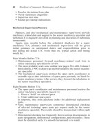
is the so-called Weibull modulus; it can be read
from a graphical representation of (2.1). Low values for m indicate a large intrinsic
variability in particle strength. A Weibull plot for aluminium oxide abrasive par-
ticles, based on the results of compressive crushing tests, is displayed in Fig. 2.1.
Values for the Weibull modulus estimated for different abrasive materials are listed

in Table 2.5. There is a notable trend in the values that both fracture strength and
Weibull modulus drop with increasing particle size. Therefore, scatter in strength
of abrasive particles can be assumed to be wider for larger particles. The relation-
ship between abrasive particle size and fracture strength of the particles is shown in
Fig. 2.2. This phenomenon can be explained through the higher absolute number of
defects in larger particles. The probability that a defect with a critical dimension (for
example, a critical crack length in a fracture mechanics approach) exists increases
with an increasing number of defects.
This effect was also observed by Larssen-Basse (1993). This author found also
that the Weibull modulus of abrasive particles depended on the atmospheric humid-
ity. Larssen-Basse (1993) performed crushing tests with SiC-particles, and he found
that, if humidity increased, the Weibull modulus and the number of fragments both
2.2 Abrasive Material Structure and Hardness 9
Table 2.2 Selected abrasive properties (References: manufacturer data)
Brand name Bulk density
a
in
t/m
3
Apparent density
in t/m
3
Hardness
b–e
Melting point in
◦
C
Grain size
min–max in mm
Major composite

in %
Technical name
Abrablast – 4.3 9
b
1,900 – Al
2
O
3
(71.9) Zirconium corundum
Abramax 1.0–2.0 3.95 2,200
c
2,000 – Al
2
O
3
(99.6) Corundum
Abrasit 1.1–2.3 3.96 2,100
c
2,000 – Al
2
O
3
(96.4) Corundum
Afesikos 1.4 2.6 8
b
– 0.04–1.4 SiO
2
(53) Aluminium silica
Afesikos HS 2.83 4.1 8
b

– 0.04–1.4 SiO
2
(36) Garnet
Afesikos SK 1.8 3.96 9
b
– 0.06–2.8 Al
2
O
3
(99.3) Corundum
Asilikos 1.3 2.5–2.6 7–8
b
– 0.06–2.8 SiO
2
(51) Aluminium silica
Cast steel – – 60
d
– 0.12–3.36 – –
Garnet – 3.9–4.1 8–9
b
1,315 – SiO
2
(41.3) Garnet
Glass beads 1.5 2.45 6
b
– 0.07–0.4 SiO
2
(73) –
GSR 3.7–4.3 7.4 44–58
d

– 0.1–2.24 – Cast steel
Cast iron 2.7–4.3 7.4 56–64
d
–upto3.15––
Ceramic spheres 2.3 3.8 60–65
d
– 0.07–0.25 ZrO
2
(67) Ceramics
MKE 1.75 3.92 1,800–2,200
e
– 0.001–2.8 Al
2
O
3
(99.6) Corundum
Olivine 1.7–1.9 5.3 6.5–7
b
1,760 0.09–1.0 MgO (50) –
Scorex 1.35 – – – 0.5–2.8 SiO
2
(40) Refinery slag
Steel grit – 7.5 48–66
d
– 0.2–1.7 – –
Steel shot – 7.3 46–51
d
– 0.2–2.0 – –
Testra 1.2–1.4 2.5–2.7 7
b

– 0.09–2.0 SiO
2
(54) Melting chamber slag
a
Depends on grain size
Hardness parameter:
b
Mohs;
c
Vickers;
d
Rockwell;
e
Knoop
10 2 Abrasive Materials
Table 2.3 Structural properties of abrasive materials (Vasek et al., 1993)
Material Damaged grains (%) Lattice constant (
˚
A) Cell volume (
˚
A
3
)
Almandine 5–60 11.522 (0.006) 1,529.62
Spessartine – 11.613 (0.005) 1,566.15
Pyrope – 11.457 (0.005) 1,503.88
Grossular 30 11.867 (0.005) 1,671.18
Andradite 80–90 12.091 (0.009) 1,767.61
increased. This feature can be attributed to moisture-assisted sharpening of the tips
of surface defects present in the particles.

The presence of defects, such as cracks and voids, affects the cleaning and
degradation performance of abrasive materials. Number and size of defects are,
Table 2.4 Data sheet for a garnet blast cleaning abrasive material (Reference: GMA Garnet)
Parameter Value
Average chemical composition
SiO
a
2
36%
Al
2
O
3
20%
FeO 30%
Fe
2
O
3
2%
TiO
2
1%
MnO 1%
CaO 2%
MgO 6%
Physical characteristics
Bulk density 2,300 kg/m
3
Specific gravity 4.1

Hardness (Mohs) 7.5–8
Melting point 1,250
◦
C
Grain shape Sub-angular
Other characteristics
Conductivity 10–15 mS/m
Moisture absorption Non-hydroscopic
Total chlorides 10–15 ppm
Ferrite (free iron) <0.01%
Lead <0.002%
Copper <0.005%
Other heavy metals <0.01%
Sulphur <0.01%
Mineral composition
Garnet (Almandine) 97–98%
Ilmenite 1–2%
Zircon 0.2%
Quartz (free silica) <0.5%
Others 0.25%
a
Refers to SiO
2
bound within the lattice of the homo-
geneous garnet crystal (no free silica)
2.2 Abrasive Material Structure and Hardness 11
Fig. 2.1 Weibull plot for the strength of aluminium oxide particles (Verspui et al., 1997). Abrasive
particle size: 10–500 μm
therefore, important assessment criteria. Cast steel shot, for example, should not
contain cracked particles, as illustrated in Fig. 2.3, in excess of 15%. Cast steel

grit should not contain cracked particles, as shown in Fig. 2.4, in excess of 40%
(SFSA, 1980). Requirements for the defects of particles of metallic abrasive mate-
rials are listed in Table 2.6.
Table 2.5 Strength parameters for abrasive materials (Yashima et al., 1987; Huang et al., 1995)
Abrasive material Grain size
in mm
Fracture strength
in MPa
Weibull
modulus
∗
a
in
MPa/mm
3
Brown corundum 2.58 67.5 1.98 228.8
1.85 78.6 2.47 142.8
1.29 115.4 2.88 135.1
0.78 200.5 3.47 149.0
Rounded corundum 1.85 96.1 3.41 160.8
White corundum 1.29 79.5 2.57 127.3
Sintered corundum 1.85 110.8 3.85 174.9
Green silicon carbide 1.85 62.2 1.92 155.5
Quartz 0.1–2.0 – 21.0 –
Glass beads – – 5.90 –
a
Defect distribution parameter
12 2 Abrasive Materials
Fig. 2.2 Relationship between abrasive particle size and particle fracture strength (values from
Huang et al., 1995)

Fig. 2.3 Cracks in cast steel shot particles; magnification: 10× (SFSA, 1980)
2.2 Abrasive Material Structure and Hardness 13
Fig. 2.4 Cracks in cast steel grit particles; magnification: 10× (SFSA, 1980)
2.2.2 Hardness of Abrasive Materials
The hardness of abrasive materials is usually estimated by two types of tests:
a scratching test for non-metallic abrasive materials, which delivers the Mohs
hardness, and indentation tests for metallic materials, which deliver either the
Knoop hardness or the Vickers hardness. Respective values for commercial abrasive
materials are listed in Table 2.2.
Mohs hardness is based on a scale of ten minerals, which is provided in Table 2.7.
The hardness of a material is measured against the scale by finding the hardest
Table 2.6 Particle defect requirements for metallic abrasive materials (ISO 11124/2-4)
Property Chilled iron grit High-carbon cast
steel shot
High-carbon cast
steel grit
Low-carbon
cast steel shot
Particle shape Max. 10% shot
or more than
half-round
Max. 5%
non-round
Max. 10% shot or more
than half-round for
grit up to 700 HV;
max. 5% for grit
above 700 HV
Max. 5%
non-round

Voids Max. 10% Max. 10% Max. 10% Max. 15%
Shrinkage
defects
Max. 10% Max. 10% Max. 10% Max. 5%
Cracks Max. 40% Max. 15% Max. 40% None
Total defects Max. 40% Max. 20% Max. 40% Max. 20%
14 2 Abrasive Materials
Table 2.7 Mohs scale (Tabor, 1951)
Material Mohs hardness
Talc 1
Gypsum 2
Calcite 3
Fluorite 4
Apatite 5
Orthoclase (Feldspar) 6
Quartz 7
Topaz 8
Corundum 9
Diamond 10
material that the given material can scratch, and/or the softest material that can
scratch the given material. For example, if some material is scratched by quartz
but not by feldspar, its hardness on Mohs scale is 6.5. In abrasive standardisation,
abrasive particles are being rubbed against a glass plate having a Mohs hardness
corresponding to 7. If the particles can scratch the plate, their hardness is >Mohs 7.
If they do not scratch the plate, their hardness is <Mohs 7. It is because of this pro-
cedure that data sheets for mineral abrasive materials often list the Mohs hardness
as >7 only.
The principles of two frequently applied indentation hardness tests are illus-
trated in Table 2.8. In laboratory practice, an abrasive particle is embedded in
a special resin matrix, and it is then being polished in order to obtain an even

Table 2.8 Indentation hardness measurement methods (Images: TWI, Cambridge, UK)
Method Brinell Vickers
Principle
Measurement
Calculation
a
H
B
=
F
π
2
· D ·

D −(D
2
− d
2
)
1/2

H
V
=
2 ·F · sin (136
◦
/2)
d
2
a

F= indentation load
d = indentation size =
d
1
+ d
2
2
D = indenter size
2.2 Abrasive Material Structure and Hardness 15
(a)
(b)
Fig. 2.5 Vickers hardness distributions of two cut wire samples (Gesell, 1979). (a) Laboratory
sample; (b) Work sample
16 2 Abrasive Materials
smooth cross-section where the actual indentation test is being performed. In-
dentation hardness values are always dependent on indentation load, and care
should be taken to provide the certain applied indentation load in data sheets.
Values from indentation hardness tests and from Mohs hardness tests can be re-
lated to each other; exceptions are diamond and corundum (Bowden and Ta-
bor, 1964).
The hardness of metallic abrasive particles is a probabilistic parameter, and the
hardness values mentioned in data sheets are mainly mean values only. Two typ-
ical abrasive hardness distribution diagrams of cut wire samples are provided in
Fig. 2.5. Figure 2.5a shows the distribution of a laboratory sample, whereas Fig. 2.5b
illustrates the distribution of a working sample. Although both materials had equal
hardness designations of 420 HV, the distributions differed widely. The laboratory
sample had a unimodal distribution with a maximum at a Vickers hardness of about
430 HV, whereas the working sample featured a multimodal distribution. The hard-
ness distribution of the laboratory sample can be expressed through a Normal dis-
tribution – this is shown in Fig. 2.6. This result points to a rather homogeneous

response of the wire material to the indentation with the Vickers pyramid, which is
not always the case (Lange and Schimm¨oller, 1967). Such a distribution was also
reported by Flavenot and Lu (1990) for steel wire shot.
Fig. 2.6 Normal distribution function for the laboratory cut wire sample plotted in Fig. 2.5a
2.3 Abrasive Particle Shape Parameters 17
2.3 Abrasive Particle Shape Parameters
2.3.1 Basic Shape Definitions
The following three basic shape definitions are provided for abrasive particles used
for blast cleaning applications:
r
shot;
r
grit;
r
cylindrical.
The corresponding designations are listed in Table 2.9. Examples for two shape
definition are displayed in Fig. 2.7. The term shot characterises grains with a pre-
dominantly spherical shape. Their length-to-diameter ratio is <2, and they do not
exhibit sharp edges or broken sections. The term grit characterises grains with a
predominantly angular shape. These grains exhibit sharp edges and broken sections.
The term cylindrical denotes grains that are manufactured by a cutting process. Their
length-to-diameter ratiois ∼1. This shapecanonlybefound with cut steel wire pellets.
2.3.2 Relative Proportions of Particles
Shape parameters characterise the shape of individual particles. Wadell (1933) and
Heywood (1933) were probably the first who gave rigorous analyses of shape
parameters. Heywood (1933)considered the shape of a particle to have the following
two distinct characteristics:
r
the relative proportions of length, breadth and thickness;
r

the geometrical form.
The relative proportion includes two parameters: (1) the elongation ratio (r
E
)and
(2) the flatness ratio (r
F
). Both parameters are defined and illustrated in Table 2.10.
Bahadur and Badruddin (1990) applied the elongation ratio to investigate the in-
fluence of the abrasive particle shape on particle impact erosion processes. They
found notable relationships between abrasive type, abrasive particle diameter and
abrasive particle shape. Some results of their study are provided in Fig. 2.8. Silica
carbide particles became more elongated and less circular with an increase in the
particle size, while the opposite was the case with aluminium oxide particles. The
general variation of silica oxide was similar to that of silica carbide particles, though
not as systematic. The elongation ratios for the silica carbide particles and for the
Table 2.9 Grain shape designations
Designation Grain shape Symbol
Shot Spherical, round S
Grit Angular, irregular G
Cylindrical Sharp-edged C
18 2 Abrasive Materials
(a)
(b)
Fig. 2.7 Basic shape designations for abrasive particles (Photographs: Kuhmichel GmbH).
(a) Grit; (b) Shot
aluminium oxide were very sensitive to the particle size in the range of small parti-
cles. For equal grain sizes, silica oxide particles featured much higher elongation
ratios than silica carbide particles. For a particle diameter of d
P
= 300 μm, as

an example, the elongation ratio was r
E
= 0.53 for silica carbide, and r
E
= 0.7
for silica oxide. A relationship between particle abrasive size and shape was also
noted by Djurovic et al. (1999). For starch media, these authors found that smaller
particles were less elongated than larger particles. These results clearly show that
particle shape may be considered an abrasive material characteristic.
2.3.3 Geometrical Forms of Particles
The geometrical form is a volumetric shape factor, representing the degree to which
a particle approximates an ideal geometric form (cube, sphere or tetrahedron). The
following two parameters can describe the geometrical form of particles: (1) the
sphericity (S
P
) and (2) the roundness (S
R
).
2.3 Abrasive Particle Shape Parameters 19
Table 2.10 Shape parameters for abrasive particles
Parameter and definition Graphical expression
Shape factor
F
shape
=
d
min
d
max
Circularity factor

F
0
=
4 · π · A
P
Perimeter
2
Roundness
S
R
=


2·r
corner
d
P

N
corner
Sphericity
S
P
=

4
π
· b
P
· l

P
d
circle
Elongation ratio
r
E
=
l
P
b
P
Flatness ratio
r
F
=
l
P
t
P
20 2 Abrasive Materials
Fig. 2.8 Relationships between abrasive material, particle size and particle shape (Bahadur and
Badruddin, 1990)
The sphericity, introduced by Wadell (1933), is defined and illustrated in
Table 2.10. In two dimensions, the sphericity is related to the projection area of
the sphere yielding the roundness, which is defined and illustrated in Table 2.10 as
well. Both sphericity and roundness range from “0” for very angular particles to “1”
for ideally round particles. Hansink (1998) defined an alternative roundness scale,
which is illustrated in Fig. 2.9, for the assessment of the shapes of abrasive particles.
This scale defines and quantifies the often used qualitative terms angularor rounded.
Several references used roundness–sphericity diagrams in order to characterise the

shape of abrasive particles. Such a roundness–sphericity diagram is illustrated in
Fig. 2.10.
Vasek et al. (1993) and Martinec (1994) suggested a circularity factor, which
was originally developed by Cox (1927), and a shape factor in order to characterise
abrasive particles. The circularity factor (F
0
) is defined and illustrated in Table 2.10.
For a perfectly round particle, circularity factor will be unity. Gillespie (1996) and
Gillespie and Fowler (1991) applied image analysis in order to estimate circularity
factors (which they called “shape factors” in their papers) for shot peening media,
and they defined any value for the circularity parameter F
0
> 0.83 as acceptable for
shot peening applications. Some of their results, featuring circularity factors for a
number of real abrasive particles, are illustrated in Fig. 2.11, and it can be seen that a
notable number of particles would not meet the critical circularity factor. Figure 2.12
shows a histogram of circularity factors based on an automatic image analysing
2.3 Abrasive Particle Shape Parameters 21
Designation Very angular Angular Sub-angular
Definition 0.5 1.5 2.5
Shape image
Designation Sub-rounded Rounded Well rounded
Definition 3.5 4.5 5.5
Shape image
Fig. 2.9 Designations for angular and rounded particle shapes (Hansink, 1998)
Fig. 2.10 Roundness-sphericity diagram for a garnet abrasive material (Reference: Bohemia
Garnet)
22 2 Abrasive Materials
0.958 0.923 0.921
0.921 0.872 0.858

0.849 0.823 0.799
0.772 0.717 0.704
Fig. 2.11 Circularity factors of steel shot particles, assessed with image processing technique
(Gillespie, 1996)
procedure. It can clearly be seen that “shape” is not a well-defined standard property
for a given abrasive material. Shape parameters in general are rather characterised
by distributions with certain statistical parameters. Typical statistical parameters for
an assessment procedure are listed in Table 2.11; the listing very well illustrates the
high number of assessment parameters delivered by an automatic image analysis
procedure.
The shape factor (F
shape
) is also defined and illustrated in Table 2.10. For circles,
the shape factor is unity. Table 2.12 lists some typical values for circularity and
shape factors for a number of different abrasive materials.
2.3 Abrasive Particle Shape Parameters 23
Fig. 2.12 Frequency distribution functions of shape factors (Gillespie and Fowler, 1991)
Table 2.11 Statistics of circularity factors of cast steel shot S-280, based on automatic image
analysis (Gillespie and Fowler, 1991)
Parameter Value
Minimum 0.487
Maximum 0.926
Median 0.898
25% quartile 0.890
75% quartile 0.906
Total value 577
Mean 0.894
Geometric mean 0.893
Harmonic mean 0.893
Sample variance 0.00083

Sample standard variation 0.029
Population variance 0.00083
Population standard variation 0.02
Standard deviation of the mean 0.0011
Relative standard error 0.0013
Skew −17, 402
Kurtosis 0.000057
24 2 Abrasive Materials
Table 2.12 Shape factors and shape characteristics of garnet abrasive materials (Vasek et al., 1993)
Mineral Subtype Shape parameter
F
0
F
shape
Almandine B 0.66 0.65
M 0.69 0.67
K 0.68 0.66
G 0.66 0.64
Grossular – 0.71 0.70
Andradite V–A 0.67 0.65
V–B 0.68 0.68
V–C 0.65 0.68
2.4 Abrasive Particle Size Distribution and Abrasive
Particle Diameter
2.4.1 Particle Size Distribution
2.4.1.1 General Definitions
In general, the term “diameter” is specified for any equidimensional particle. By
conversion, particle sizes are expressed in different units depending on the size
ranges involved. Coarse grains are measured in inches or millimetres, fine particles
in terms of screen size, very fine particles are measured in micrometer or manome-

ter. A number of “diameter” definitions are known. The diameter is defined either
in terms of some real property of the particle, such as its volume or surface area, or in
terms of behaviour of the particle in some specific circumstances, such as settling in
water under defined conditions (Kelly and Spottiswood, 1982). In the area of blast
cleaning, the particle size is usually given in mesh designation (according to the
Tyler-Standard-Screen sieve series), which barely mentions the related particle size
distributions or the shape of the particles. A regression study made to link the Tyler
sieve series to the corresponding average particle diameter delivers the following
relationship:
d
P
= 17, 479 · mesh
−1.0315
(2.2)
with a regression coefficient of 0.998. The particle diameter is in μminthis
equation. A mesh number 180 would correspond to an average particle diameter of
d
p
= 82 μm.
2.4.1.2 Sieve Analysis
Because it is impracticable to individually estimate each particle, size analysis is
carried out by dividing the particles into a number of suitably narrow size ranges.
Table 2.13 presents results of sieve analyses for abrasive particle samples used in
2.4 Abrasive Particle Size Distribution and Abrasive Particle Diameter 25
Table 2.13 Sieve analyses results for two abrasive mixtures (Metabrasive Ltd.)
Sieve size in μm Weight in %
Alumina 700 Metagrit 65
125 – 2
150 – 5
212 – 20

300 4 28
425 26 35
600 45 10
850 22.5 –
1,180 2.5 –
Total 100 100
blast cleaning. Graphically, data are conventionally presented by plotting the particle
size horizontally and the measured quantity of property vertically. Two approaches
are used to present the quantity: (1) plotting the absolute amount in each size fraction
(Fig. 2.13a) and (2) plotting the cumulative amount above or below a certain size
(Fig. 2.13b).
2.4.1.3 Particle Size Distribution Models
A number of models were developed to mathematically describe the size distribu-
tions of fine-grained comminution products, which include abrasive particles. These
models have empirical relationships, which to a greater or lesser extent were found
capable of describing comminution products size distributions. Table 2.14 lists the
most frequently used models. These equations are all of the general type:
M
0
(d
P
) = f

d
P
d
∗

n
M

(2.3)
The size modulus, d*, is an indication of an average particle diameter. When
the equation has an upper size limit, d* is in fact the maximum particle size in the
distribution. Equation (2.3) also includes a second parameter, n
M
, that is frequently
called the distribution modulus, since it is a measure of the spread of particle sizes.
The higher the value for n
M
, the more homogeneous is the grain size structure of
the sample. For n
M
→∞, the sample consists of grains with equal diameters.
Figure 2.14a, b shows fits for the sieve analysis from Table 2.13 by two common
particle-size distribution functions. The Rosin–Rammler–Sperling–Bennett(RRSB)
distribution is of particular interest because its distribution parameters are utilised
by some authors as a measure of the ageing and reusability of metallic abrasive
particles (Wellinger et al., 1962).
26 2 Abrasive Materials
(a)
100
80
60
40
accumulated weight in %
sieve size in mm
alumina 700
d
p50
-line

Metagrit 65
20
0
0
0.3 0.6 0.9 1.2
(b)
Fig. 2.13 Graphical representations of sieve analysis results (see Table 2.13). (a) Absolute distri-
bution; (b) Cumulative distribution
2.4 Abrasive Particle Size Distribution and Abrasive Particle Diameter 27
Table 2.14 Particle-size distribution functions (Kelly and Spottiswood, 1982; Schubert, 1988)
Function Formula M
0
(d
P
) Significance of d* Equation
Logarithmic probability erf

ln
d
P
d
∗
σ

Medium particle diameter 2.3a
Rosin–Rammler–Sperling–
Bennett (RRSB)
1 −exp



d
P
d
∗

n
M

Particle diameter at M
0
= 63.2% 2.3b
Gates–Gaudin–Schumann
(GGS)

d
P
d
∗

n
M
2.3c
Gaudin–Meloy 1 −

1 −
d
P
d
∗


2
Maximum particle diameter 2.3d
Broadbent–Callcott
1−exp

−
d
P
d
∗

1−exp(−1)
–2.3e
2.4.2 Particle Diameter
According to regulations in ISO 1117, the particle diameter is defined according to
a particle “size class”. A size class of “140”, for example, means a particle diameter
of 1.4 mm.
If the particle size distribution is known from the sieve analysis, several “average”
diameter values of the particle sample can be estimated. The median diameter, d
50
,
is the 50% point on any cumulative distribution curve (Fig. 2.13b). For the examples
presented in Table 2.13 and Fig. 2.13, this diameter is d
P50
= 510 μm (Alumina 700)
and d
P50
= 280 μm (MG 65), respectively. The geometric mean diameter, d
PG
,is

based on the assumption of an even graduation in size from maximum to minimum,
and it assumes an equal number of particles in each size average:
d
PG
=
d
Pmax
+ d
Pmin
2
(2.4)
In the examples given in Table 2.13 and Fig. 2.13, this diameter is d
PG
= 740 μm
(Alumina 700) and d
PG
= 362 μm (MG 65), respectively. A third approach is the
definition of a statistical diameter, d
PSt
, which follows the equation:
d
PSt
=

n
i=1
(m
i
· d
Pi

)
100
(2.5)
For the examples in Table 2.13 and Fig. 2.13, the statistical diameter is d
PSt
=613 μm
(Alumina 700) and d
PSt
= 345 μm (MG 65), respectively.
2.4.3 Alternative Abrasive Particle Size Assessment Methods
Particle sizes, but also particle size distributions, can be assessed also by ap-
plying image analysis methods. This alternative approach is not a standard in
28 2 Abrasive Materials
(a)
2
In (sieve size in mm)
f (sieve size )
alumina 700
Metagrit
output
0
–4
–2
–2.4 –1.6 –0.8
0
(b)
Fig. 2.14 Distribution functions for sieve analysis results (see Table 2.12). (a) Gates–Gaudin–
Schumann (GGS) distribution; (b) Rosin–Rammler–Sperling–Bennett (RRSB) distribution
2.4 Abrasive Particle Size Distribution and Abrasive Particle Diameter 29
the blast cleaning industry, although promising results have been reported for

the image analysis of shot peening media. Gillespie (1996) and Gillespie and
Fowler (1991) performed comparative size measurements by using conventional
sieve analysis, a digital micrometer and image analysis. Some results are dis-
played in Fig. 2.15. The agreement between the three methods depended on the
sieve size; it was very good (less than 2 wt.%) for the smaller sieve sizes. The
average difference between sieve analysis and image analysis was 2.71 wt.%. Im-
age analysis is of definite interest because this method can deliver information
on particle size as well as on particle shape. Promising experience is available
on the shape assessment of particles, either of shot peening media (Gillespie and
Fowler, 1991; Gillespie, 1996) or of erosion debris (Momber and Wong, 2005b),
with image analysis methods. Further details on this application are provided in
Sect. 2.3.
Optical methods for the assessment of particle sizes are very familiar in particle
technology. Sparks and Hutchings (1993) have, however, shown that these methods
must be applied with caution to broken abrasive particles. Especially glass particles
show different optical properties whether they are round (e.g. glass beads) or broken
(e.g. glass grit). Broken glass particles would, in a correct orientation with respect
to a laser beam, diffract light in such a way so as to suggest that they were of larger
diameter.
Fig. 2.15 Comparison between abrasive size assessment methods (Gillespie, 1996)
30 2 Abrasive Materials
2.5 Density of Abrasive Materials
The following two density parameters are defined for abrasives:
r
apparent density;
r
bulk density.
The apparent density is the ratio between mass and volume of a single abrasive
grain:
ρ

P
=
m
P
V
P
=
6 · m
P
π · d
3
P
(2.6)
It can be estimated with well-defined methods. This density parameter includes
flaws, pores and cracks. Therefore, it is a physical constant of the material. The
apparent density must, for example, be used if kinetic energy of an impinging grain
is calculated.
The bulk density is the mass of a volume of a group of individual grains. Bulk
density depends on packing density of the grain sample. It is affected, for example,
by grain size and grain shape. Exactly seen, it is not a material property. However,
some values for typical blasting media are listed in Table 2.2, based on standard
grain samples. A typical ratio between apparent density and bulk density is ∼2for
many abrasive materials.
2.6 Number and Kinetic Energy of Abrasive Particles
2.6.1 Abrasive Particle Number and Frequency
The number of particles involved in a blast cleaning process can be approximated
as follows:
N
P
=

˙m
P
m
P
· t
E
(2.7)
The mass of an individual abrasive particle is:
m
P
=
π
6
· d
3
P
· ρ
P
(2.8)
for spherical particles. If, for example, the median particle diameter d
P50
is utilised,
the number of particles in a transversal (y-direction) moving blast cleaning jet is:
N
P
=
6 · ˙m
P
· y
π · ρ

P
· d
3
P50
· v
T
(2.9)
2.6 Number and Kinetic Energy of Abrasive Particles 31
For a given traverse distance, the higher the abrasive mass flow rate, the higher
the number of abrasive particles. The higher the abrasive material density and av-
erage abrasive particle diameter, the lower the number of abrasive particles. The
abrasive particle impact frequency is simply:
˙
N
P
=
N
P
t
E
=
˙m
P
m
P
(2.10)
For a given exposure time, the impact frequency increases with an increase in
abrasive mass flow rate and with a decrease in average particle diameter. If abrasive
material density increases, the impact frequency decreases. Henning and Brauer
(1986) introduced a particle frequency number:

˙n
P
=
˙
N
P
A
C
(2.11)
which considers geometrical effects. The unit of this parameter is 1/(s ·m
2
). Glatzel
and Brauer (1978) defined a dimensionless collision number, which characterised
the collision between reflected and incident abrasive particles:
c
K
=
c
R
· d
N
d
P
· cos ϕ
(2.12)
The variable c
R
is the particle concentration in the impinging stream. This vari-
able can be calculated as follows:
c

R
=
4
π
·
˙m
P
v
P
· ρ
P
· d
2
N
(2.13)
The collision number is high for a high particle concentration, for a small nozzle
diameter, for small abrasive particles, and for high angles of impingement.
2.6.2 Kinetic Energy of Abrasive Particles
The kinetic energy of a spherical abrasive particle is simply:
E
P
=
π
12
· d
3
P
· ρ
P
· v

2
P
(2.14)
Data plotted in Fig. 2.16 illustrate typical values for kinetic energies. The kinetic
energy of a glass bead with a density ρ
P
= 2,450kg/m
3
, a diameter d
P
= 1.5mm and
an impingement velocity v
P
= 100 m/s reads E
P
= 0.022 J as marked in the graph.
It may, however, be noted that abrasive particle size and abrasive particle velocity
cannot be varied independently on each other in most blast cleaning devices. This
special topic is discussed in Sect. 3.6.3. The power delivered to the cleaning site by