Computational Physics - M. Jensen Episode 1 Part 8 pdf
Bạn đang xem bản rút gọn của tài liệu. Xem và tải ngay bản đầy đủ của tài liệu tại đây (315.76 KB, 20 trang )
9.1. INTRODUCTION 129
Eleven new attempts may results in a totally different sequence of numbers and so forth. Repeat-
ing this exercise the next evening, will most likely never give you the same sequences. Thus, we
say that the outcome of this hobby of ours is truly random.
Random variables are hence characterized by a domain which contains all possible values
that the random value may take. This domain has a corresponding PDF.
To give you another example of possible random number spare time activities, consider the
radioactive decay of an
-particle from a certain nucleus. Assume that you have at your disposal
a Geiger-counter which registers every say 10ms whether an -particle reaches the counter or
not. If we record a hit as 1 and no observation as zero, and repeat this experiment for a long time,
the outcome of the experiment is also truly random. We cannot form a specific pattern from the
above observations. The only possibility to say something about the outcome is given by the
PDF, which in this case the well-known exponential function
(9.5)
with being proportional with the half-life.
9.1.1 First illustration of the use of Monte-Carlo methods, crude integra-
tion
With this definition of a random variable and its associated PDF, we attempt now a clarification
of the Monte-Carlo strategy by using the evaluation of an integral as our example.
In the previous chapter we discussed standard methods for evaluating an integral like
(9.6)
where
are the weights determined by the specific integration method (like Simpson’s or Tay-
lor’s methods) with the given mesh points. To give you a feeling of how we are to evaluate the
above integral using Monte-Carlo, we employ here the crudest possible approach. Later on we
will present slightly more refined approaches. This crude approach consists in setting all weights
equal 1,
. Recall also that where , in our case and is
the step size. We can then rewrite the above integral as
(9.7)
but this is nothing but the average of
over the interval [0,1], i.e.,
(9.8)
In addition to the average value
the other important quantity in a Monte-Carlo calculation
is the variance or the standard deviation . We define first the variance of the integral with
130 CHAPTER 9. OUTLINE OF THE MONTE-CARLO STRATEGY
to be
(9.9)
or
(9.10)
which is nothing but a measure of the extent to which
deviates from its average over the region
of integration.
If we consider the results for a fixed value of
as a measurement, we could however re-
calculate the above average and variance for a series of different measurements. If each such
measumerent produces a set of averages for the integral
denoted , we have for mea-
sumerements that the integral is given by
(9.11)
The variance for these series of measurements is then for
(9.12)
Splitting the sum in the first term on the right hand side into a sum with
and one with
we assume that in the limit of a large number of measurements only terms with survive,
yielding
(9.13)
We note that
(9.14)
The aim is to have as small as possible after samples. The results from one sample
represents, since we are using concepts from statistics, a ’measurement’.
The scaling in the previous equation is clearly unfavorable compared even with the trape-
zoidal rule. In the previous chapter we saw that the trapezoidal rule carries a truncation error
, with the step length. In general, methods based on a Taylor expansion such as the
trapezoidal rule or Simpson’s rule have a truncation error which goes like , with .
Recalling that the step size is defined as , we have an error which goes like .
However, Monte Carlo integration is more efficient in higher dimensions. To see this, let
us assume that our integration volume is a hypercube with side
and dimension . This cube
contains hence points and therefore the error in the result scales as for the
traditional methods. The error in the Monte carlo integration is however independent of
and
scales as , always! Comparing this error with that of the traditional methods, shows
that Monte Carlo integration is more efficient than an order-k algorithm when .
9.1. INTRODUCTION 131
Below we list a program which integrates
(9.15)
where the input is the desired number of Monte Carlo samples. Note that we transfer the variable
in order to initialize the random number generator from the function . The variable
gets changed for every sampling. This variable is called the seed.
What we are doing is to employ a random number generator to obtain numbers
in the in-
terval through e.g., a call to one of the library functions , , . These functions
will be discussed in the next section. Here we simply employ these functions in order to generate
a random variable. All random number generators produce in a pseudo-random form numbers in
the interval
using the so-called uniform probability distribution defined as
(9.16)
with
og . If we have a general interval , we can still use these random number
generators through a variable change
(9.17)
with
in the interval .
The present approach to the above integral is often called ’crude’ or ’Brute-Force’ Monte-
Carlo. Later on in this chapter we will study refinements to this simple approach. The reason for
doing so is that a random generator produces points that are distributed in a homogenous way in
the interval
. If our function is peaked around certain values of , we may end up sampling
function values where is small or near zero. Better schemes which reflect the properties of
the function to be integrated are thence needed.
The algorithm is as follows
Choose the number of Monte Carlo samples .
Perform a loop over and for each step generate a a random number in the interval
trough a call to a random number generator.
Use this number to evaluate .
Evaluate the contributions to the mean value and the standard deviation for each loop.
After samples calculate the final mean value and the standard deviation.
The following program implements the above algorithm using the library function
. Note
the inclusion of the file.
132 CHAPTER 9. OUTLINE OF THE MONTE-CARLO STRATEGY
# include < iostream >
# include
using namespace st d ;
/ / Here we de fi ne v ari ous f un c ti on s c al le d by the main program
/ / t h is f un c ti on de fi ne s the f un ct io n to i nt e gr a te
double func ( double x) ;
/ / Main fu nc ti on begins here
in t main ()
{
in t i , n ;
long idum ;
double crude_mc , x , sum_sigma , fx , v ari anc e ;
cout < < < < endl ;
cin > > n ;
crude_mc = sum_sigma = 0 . ; idum = 1 ;
/ / ev alu ate the in t eg r a l with the a crude Monte Carlo method
for ( i = 1 ; i <= n ; i ++){
x=ran0 (&idum ) ;
fx=func (x ) ;
crude_mc += fx ;
sum_sigma + = fx fx ;
}
crude_mc = crude_mc / ( ( double ) n ) ;
sum_sigma = sum_sigma / ( ( double ) n ) ;
va ria nce =sum_sigma crude_mc crude_mc ;
/ / f i n a l out put
cout < < < < va ria nce < <
<< crude_mc < < < < M_PI /4. < < endl ;
} / / end of main program
/ / th i s fu nc ti on d e fin e s the f un ct io n t o i nte g ra t e
double func ( double x )
{
double value ;
value = 1 . / ( 1 . + x x ) ;
return val ue ;
} / / end of f un ct io n t o eval uate
9.1. INTRODUCTION 133
The following table list the results from the above program as function of the number of Monte
Carlo samples.
Table 9.1: Results for
as function of number of Monte Carlo samples .
The exact answer is
with 6 digits.
10 7.75656E-01 4.99251E-02
100 7.57333E-01 1.59064E-02
1000 7.83486E-01 5.14102E-03
10000 7.85488E-01 1.60311E-03
100000 7.85009E-01 5.08745E-04
1000000 7.85533E-01 1.60826E-04
10000000 7.85443E-01 5.08381E-05
We note that as increases, the standard deviation decreases, however the integral itself
never reaches more than an agreement to the third or fourth digit. Improvements to this crude
Monte Carlo approach will be discussed.
As an alternative, we could have used the random number generator provided by the compiler
through the function
, as shown in the next example.
/ / crude mc fu nc ti on to c al cul at e pi
# include < iostream >
using namespace s td ;
in t main ()
{
const in t n = 1000000;
double x , fx , pi , in ver s_p eriod , pi2 ;
in t i ;
i nv er s_ pe ri od = 1 . /RAND_MAX;
srand ( time (NULL) ) ;
pi = pi2 = 0 . ;
for ( i = 0; i <n ; i ++)
{
x = double ( rand ( ) ) in ve rs _p er io d ;
fx = 4 . / ( 1 + x x ) ;
pi + = fx ;
pi2 + = fx fx ;
}
pi / = n ; pi2 = pi2 / n pi pi ;
134 CHAPTER 9. OUTLINE OF THE MONTE-CARLO STRATEGY
cout < < < < pi < < < < pi2 < < endl ;
return 0 ;
}
9.1.2 Second illustration, particles in a box
We give here an example of how a system evolves towards a well defined equilibrium state.
Consider a box divided into two equal halves separated by a wall. At the beginning, time
, there are particles on the left side. A small hole in the wall is then opened and one
particle can pass through the hole per unit time.
After some time the system reaches its equilibrium state with equally many particles in both
halves,
. Instead of determining complicated initial conditions for a system of particles,
we model the system by a simple statistical model. In order to simulate this system, which may
consist of
particles, we assume that all particles in the left half have equal probabilities
of going to the right half. We introduce the label to denote the number of particles at every
time on the left side, and for those on the right side. The probability for a move
to the right during a time step
is . The algorithm for simulating this problem may then
look like as follows
Choose the number of particles .
Make a loop over time, where the maximum time should be larger than the number of
particles
.
For every time step there is a probability for a move to the right. Compare this
probability with a random number
.
If , decrease the number of particles in the left half by one, i.e., .
Else, move a particle from the right half to the left, i.e.,
.
Increase the time by one unit (the external loop).
In this case, a Monte Carlo sample corresponds to one time unit .
The following simple C-program illustrates this model.
/ / P a rt i cl e s in a box
# include < iostream >
# include < fstream >
# include < iomanip >
# include
using namespace st d ;
ofstream o f i l e ;
in t main ( in t argc , char argv [ ] )
{
9.1. INTRODUCTION 135
char out fil ena me ;
in t i n i t i a l _ n _ p a r t i c l e s , max_time , time , random_n , n l e f t ;
long idum ;
/ / Read in o utp ut f i l e , abort i f the re are too few command l i ne
arguments
i f ( argc <= 1 ) {
cout < < < < argv [0] < <
< < endl ;
e xi t ( 1) ;
}
e ls e {
outfi len am e=argv [ 1 ] ;
}
o f i l e . open ( o utf ile nam e ) ;
/ / Read in data
cout < < < < endl ;
cin > > i n i t i a l _ n _ p a r t i c l e s ;
/ / setup of i n i t i a l co nd it ion s
n l e f t = i n i t i a l _ n _ p a r t i c l e s ;
max_time = 10 i n i t i a l _ n _ p a r t i c l e s ;
idum = 1;
/ / sampling over number of p a r t i cl e s
for ( time =0 ; time <= max_time ; time ++){
random_n = ( ( i nt ) i n i t i a l _ n _ p a r t i c l e s ran0 (&idum ) ) ;
i f ( random_n <= n l e f t ) {
n l e f t = 1;
}
els e {
n l e f t + = 1 ;
}
o f i l e < < s e t i o s f l a g s ( io s : : showpoint | io s : : uppercase ) ;
o f i l e < < setw (15) < < time ;
o f i l e < < setw (15) < < n l e f t < < endl ;
}
return 0 ;
} / / end main fu nc ti on
The enclosed figure shows the development of this system as function of time steps. We note
that for
after roughly time steps, the system has reached the equilibrium state.
There are however noteworthy fluctuations around equilibrium.
If we denote as the number of particles in the left half as a time average after equilibrium
is reached, we can define the standard deviation as
(9.18)
This problem has also an analytic solution to which we can compare our numerical simula-
136 CHAPTER 9. OUTLINE OF THE MONTE-CARLO STRATEGY
Figure 9.1: Number of particles in the left half of the container as function of the number of time
steps. The solution is compared with the analytic expression. .
tion. If
are the number of particles in the left half after moves, the change in in the
time interval is
(9.19)
and assuming that
and are continuous variables we arrive at
(9.20)
whose solution is
(9.21)
with the initial condition .
9.1.3 Radioactive decay
Radioactive decay is among one of the classical examples on use of Monte-Carlo simulations.
Assume that a the time
we have nuclei of type which can decay radioactively. At
a time we are left with nuclei. With a transition probability , which expresses the
probability that the system will make a transition to another state during oen second, we have the
following first-order differential equation
(9.22)
9.1. INTRODUCTION 137
whose solution is
(9.23)
where we have defined the mean lifetime
of as
(9.24)
If a nucleus
decays to a daugther nucleus which also can decay, we get the following
coupled equations
(9.25)
and
(9.26)
The program example in the next subsection illustrates how we can simulate such a decay process
through a Monte Carlo sampling procedure.
9.1.4 Program example for radioactive decay of one type of nucleus
The program is split in four tasks, a main program with various declarations,
/ / Ra dio act iv e decay of nu cl ei
# include < iostream >
# include < fstream >
# include < iomanip >
# include
using namespace st d ;
ofstream o f i l e ;
/ / Function t o read in data from screen
void i n i t i a l i s e ( i nt & , in t & , in t & , double & ) ;
/ / The Mc sampling for nuclear decay
void mc_sampling ( int , int , int , double , int ) ;
/ / p r in t s to sc reen the r e sul t s of the c a lc u la t io n s
void output ( int , int , int ) ;
in t main ( in t argc , char argv [ ] )
{
char out fil ena me ;
in t i n i t i a l _ n _ p a r t i c l e s , max_time , number_cycles ;
double de ca y_ prob ab il it y ;
in t ncum ulat ive ;
/ / Read in o utp ut f i l e , abort i f the re are too few command l i ne
arguments
i f ( argc <= 1 ) {
cout < < < < argv [0] < <
138 CHAPTER 9. OUTLINE OF THE MONTE-CARLO STRATEGY
< < endl ;
e xi t ( 1) ;
}
e ls e {
outfi len am e=argv [ 1 ] ;
}
o f i l e . open ( o utf ile nam e ) ;
/ / Read in data
i n i t i a l i s e ( i n i t i a l _ n _ pa rt i c l e s , max_time , number_cycles ,
dec ay _p ro bab il it y ) ;
ncumulati ve = new i nt [ max_time +1];
/ / Do the mc sampling
mc_sampling ( i n i t i a l _ n _ p a r t i c l e s , max_time , number_cycles ,
de cay _pr ob abil it y , ncumulative ) ;
/ / Pr int out r e s u l ts
outpu t ( max_time , number_cycles , ncumul ative ) ;
de le te [ ] ncumul ative ;
return 0 ;
} / / end of main fu nc ti on
the part which performs the Monte Carlo sampling
void mc_sampling ( i nt i n i t i a l _ n _ p a r t i c l e s , in t max_time ,
in t number_cycles , double dec ay_ pro ba bi li ty ,
in t ncumulative )
{
in t cycles , time , np , n_unstable , p a r t i c l e _ l i m i t ;
long idum ;
idum = 1; / / i n i t i a l i s e random number generator
/ / loop over monte carlo cy cl es
/ / One monte carlo loop i s one sample
for ( c ycl es = 1 ; cy cl es <= number_cycles ; cyc les ++){
n_unstab le = i n i t i a l _ n _ p a r t i c l e s ;
/ / accumulate the number of pa r t i c l es per time ste p per t r i a l
ncumulati ve [ 0] + = i n i t i a l _ n _ p a r t i c l e s ;
/ / loop over each time st ep
for ( time =1 ; time <= max_time ; time ++){
/ / fo r each time step , we check each p a r ti c l e
p a r t i c l e _ l i m i t = n_ uns tab le ;
for ( np = 1 ; np <= p a r t i c l e _ l i m i t ; np ++) {
i f ( ran0 (&idum ) <= d ec ay _p roba bi li ty ) {
n_unstab le =n_unstabl e 1;
}
} / / end of loop over p a rt i c l es
ncumulati ve [ time ] + = n_u nst ab le ;
9.1. INTRODUCTION 139
} / / end of loop over time st ep s
} / / end of loop over MC t r i a l s
} / / end mc_sampling f un ct io n
and finally functions for reading input and writing output data
void i n i t i a l i s e ( i nt & i n i t i a l _ n _ p a r t i c l e s , in t & max_time ,
in t & number_cycles , double & d ec ay _p ro ba bi li ty )
{
cout < < < < endl ;
cin > > i n i t i a l _ n _ p a r t i c l e s ;
cout < < < < endl ;
cin > > max_time ;
cout < < < < endl ;
cin > > number_cycles ;
cout < < < < endl ;
cin > > d ec ay _p roba bi li ty ;
} / / end of fun c ti on i n i t i a l i s e
void out put ( i nt max_time , in t number_cycles , int ncum ulative )
{
in t i ;
for ( i = 0; i <= max_time ; i ++){
o f i l e < < s e t i o s f l a g s ( io s : : showpoint | io s : : uppercase ) ;
o f i l e < < setw (15) < < i ;
o f i l e < < setw (15) < < s e tp r e c is i o n (8 ) ;
o f i l e << ncumula tive [ i ] / ( ( double ) number_cycles ) < < endl ;
}
} / / end of fun c ti on o utp ut
9.1.5 Brief summary
In essence the Monte Carlo method contains the following ingredients
A PDF which characterizes the system
Random numbers which are generated so as to cover in a as uniform as possible way on
the unity interval [0,1].
A sampling rule
An error estimation
Techniques for improving the errors
140 CHAPTER 9. OUTLINE OF THE MONTE-CARLO STRATEGY
Before we discuss various PDF’s which may be of relevance here, we need to present some
details about the way random numbers are generated. This is done in the next section. Thereafter
we present some typical PDF’s. Sections 5.4 and 5.5 discuss Monte Carlo integration in general,
how to choose the correct weighting function and how to evaluate integrals with dimensions
.
9.2 Physics Project: Decay of
Bi and Po
In this project we are going to simulate the radioactive decay of these nuclei using sampling
through random numbers. We assume that at
we have nuclei of the type which
can decay radioactively. At a given time we are left with nuclei. With a transition
rate , which is the probability that the system will make a transition to another state during a
second, we get the following differential equation
(9.27)
whose solution is
(9.28)
and where the mean lifetime of the nucleus is
(9.29)
If the nucleus
decays to , which can also decay, we get the following coupled equations
(9.30)
and
(9.31)
We assume that at
we have . In the beginning we will have an increase of
nuclei, however, they will decay thereafter. In this project we let the nucleus Bi represent
. It decays through -decay to Po, which is the nucleus in our case. The latter decays
through emision of an
-particle to Pb, which is a stable nucleus. Bi has a mean lifetime of
7.2 days while Po has a mean lifetime of 200 days.
a) Find analytic solutions for the above equations assuming continuous variables and setting
the number of
Po nuclei equal zero at .
b) Make a program which solves the above equations. What is a reasonable choice of timestep
? You could use the program on radioactive decay from the web-page of the course as
an example and make your own for the decay of two nuclei. Compare the results from
your program with the exact answer as function of
, and . Make plots
of your results.
9.3. RANDOM NUMBERS 141
c) When Po decays it produces an particle. At what time does the production of
particles reach its maximum? Compare your results with the analytic ones for ,
and .
9.3 Random numbers
Uniform deviates are just random numbers that lie within a specified range (typically 0 to 1),
with any one number in the range just as likely as any other. They are, in other words, what
you probably think random numbers are. However, we want to distinguish uniform deviates
from other sorts of random numbers, for example numbers drawn from a normal (Gaussian)
distribution of specified mean and standard deviation. These other sorts of deviates are almost
always generated by performing appropriate operations on one or more uniform deviates, as we
will see in subsequent sections. So, a reliable source of random uniform deviates, the subject
of this section, is an essential building block for any sort of stochastic modeling or Monte Carlo
computer work. A disclaimer is however appropriate. It should be fairly obvious that something
as deterministic as a computer cannot generate purely random numbers.
Numbers generated by any of the standard algorithm are in reality pseudo random numbers,
hopefully abiding to the following criteria:
1. they produce a uniform distribution in the interval [0,1].
2. correlations between random numbers are negligible
3. the period before the same sequence of random numbers is repeated is as large as possible
and finally
4. the algorithm should be fast.
That correlations, see below for more details, should be as small as possible resides in the
fact that every event should be independent of the other ones. As an example, a particular simple
system that exhibits a seemingly random behavior can be obtained from the iterative process
(9.32)
which is often used as an example of a chaotic system.
is constant and for certain values of and
the system can settle down quickly into a regular periodic sequence of values .
For and we obtain a periodic pattern as shown in Fig. 5.2. Changing to
yields a sequence which does not converge to any specific pattern. The values of
seem purely random. Although the latter choice of yields a seemingly random sequence of
values, the various values of harbor subtle correlations that a truly random number sequence
would not possess.
The most common random number generators are based on so-called Linear congruential
relations of the type
(9.33)
142 CHAPTER 9. OUTLINE OF THE MONTE-CARLO STRATEGY
100806040200
1.2
1.1
1
0.9
0.8
0.7
0.6
0.5
0.4
0.3
0.2
Figure 9.2: Plot of the logistic mapping
for and and
.
which yield a number in the interval [0,1] through
(9.34)
The number
is called the period and it should be as large as possible and is the start-
ing value, or seed. The function means the remainder, that is if we were to evaluate
, the outcome is the remainder of the division , namely .
The problem with such generators is that their outputs are periodic; they will start to repeat
themselves with a period that is at most
. If however the parameters and are badly chosen,
the period may be even shorter.
Consider the following example
(9.35)
with a seed . These generator produces the sequence , i.e.,
a sequence with period . However, increasing may not guarantee a larger period as the
following example shows
(9.36)
which still with results in , a period of just .
Typical periods for the random generators provided in the program library are of the order of
. Other random number generators which have become increasingly popular are so-called
shift-register generators. In these generators each successive number depends on many preceding
values (rather than the last values as in the linear congruential generator). For example, you could
9.3. RANDOM NUMBERS 143
make a shift register generator whose th number is the sum of the th and th values with
modulo
,
(9.37)
Such a generator again produces a sequence of pseudorandom numbers but this time with a period
much larger than
. It is also possible to construct more elaborate algorithms by including more
than two past terms in teh sum of each iteration. One example is the generator of Marsaglia and
Zaman (Computers in Physics 8 (1994) 117) which consists of two congurential relations
(9.38)
followed by
(9.39)
which according to the authors has a period larger than
.
Moreover, rather than using modular addition, we could use the bitwise exclusive-OR (
)
operation so that
(9.40)
where the bitwise action of
means that if the result is whereas if
the result is . As an example, consider the case where and . The first one
has a bit representation (using 4 bits only) which reads whereas the second number is .
Employing the
operator yields , or .
In Fortran90, the bitwise
operation is coded through the intrinsic function
where and are the input numbers, while in it is given by . The program below (from
Numerical Recipes, chapter 7.1) shows the function
which implements
(9.41)
through Schrage’s algorithm which approximates the multiplication of large integers through the
factorization
or
where the brackets denote integer division and .
Note that the program uses the bitwise
operator to generate the starting point for each
generation of a random number. The period of is . A special feature of this
algorithm is that is should never be called with the initial seed set to .
/
The f un ct io n
ran0 ( )
i s an " Minimal " random number generator of Park and M il ler
( see Numerical re cipe page 27 9) . Set or r es e t the inp ut value
idum to any i nt eg er value ( e xce pt the un l ik e l y value MASK)
144 CHAPTER 9. OUTLINE OF THE MONTE-CARLO STRATEGY
to i n i t i a l i z e the sequence ; idum must not be a lt er ed between
c a ll s f or su ce ss iv e d ev ia te s in a sequence .
The f un ct io n re tu rn s a uniform de vi at e between 0 . 0 and 1 . 0 .
/
double ran0 ( long &idum )
{
const in t a = 16 80 7 , m = 2147483647 , q = 1 277 73;
const in t r = 2 83 6 , MASK = 123459876;
const double am = 1 . /m;
long k ;
double ans ;
idum ^ = MASK;
k = ( idum ) / q ;
idum = a ( idum k q ) r k ;
i f ( idum < 0) idum + = m;
ans=am ( idum ) ;
idum ^ = MASK;
return ans ;
} / / End : fu nc ti on ran0 ( )
The other random number generators , and are described in detail in chapter 7.1
of Numerical Recipes.
Here we limit ourselves to study selected properties of these generators.
9.3.1 Properties of selected random number generators
As mentioned previously, the underlying PDF for the generation of random numbers is the uni-
form distribution, meaning that the probability for finding a number
in the interval [0,1] is
.
A random number generator should produce numbers which uniformly distributed in this
interval. Table 5.2 shows the distribution of
random numbers generated by the
functions in the program library. We note in this table that the number of points in the various
intervals
, etc are fairly close to , with some minor deviations.
Two additional measures are the standard deviation
and the mean .
For the uniform distribution with
points we have that the average is
(9.42)
and taking the limit
we have
(9.43)
9.3. RANDOM NUMBERS 145
since . The mean value is then
(9.44)
while the standard deviation is
(9.45)
The various random number generators produce results which agree rather well with these
limiting values. In the next section, in our discussion of probability distribution functions and
the central limit theorem, we are to going to see that the uniform distribution evolves towards a
normal distribution in the limit
.
Table 9.2: Number of
-values for various intervals generated by 4 random number generators,
their corresponding mean values and standard deviations. All calculations have been initialized
with the variable
.
-bin ran0 ran1 ran2 ran3
0.0-0.1 1013 991 938 1047
0.1-0.2 1002 1009 1040 1030
0.2-0.3 989 999 1030 993
0.3-0.4 939 960 1023 937
0.4-0.5 1038 1001 1002 992
0.5-0.6 1037 1047 1009 1009
0.6-0.7 1005 989 1003 989
0.7-0.8 986 962 985 954
0.8-0.9 1000 1027 1009 1023
0.9-1.0 991 1015 961 1026
0.4997 0.5018 0.4992 0.4990
0.2882 0.2892 0.2861 0.2915
There are many other tests which can be performed. Often a picture of the numbers generated
may reveal possible patterns. Another important test is the calculation of the auto-correlation
function
(9.46)
with
. Recall that . The non-vanishing of for means that
the random numbers are not independent. The independence of the random numbers is crucial
in the evaluation of other expectation values. If they are not independent, our assumption for
approximating
in Eq. (9.13) is no longer valid.
The expectation values which enter the definition of
are given by
(9.47)
146 CHAPTER 9. OUTLINE OF THE MONTE-CARLO STRATEGY
with ran1
with ran0
30002500200015001000500
0.1
0.05
0
-0.05
-0.1
Figure 9.3: Plot of the auto-correlation function
for various -values for using
the random number generators and .
Fig. 5.3 compares the auto-correlation function calculated from
and . As can be
seen, the correlations are non-zero, but small. The fact that correlations are present is expected,
since all random numbers do depend in same way on the previous numbers.
Exercise 9.1
Make a program which computes random numbers according to the algorithm of
Marsaglia and Zaman, Eqs. (9.38) and (9.39). Compute the correlation function
and compare with the auto-correlation function from the function .
9.4 Probability distribution functions
Hitherto, we have tacitly used properties of probability distribution functions in our computation
of expectation values. Here and there we have referred to the uniform PDF. It is now time to
present some general features of PDFs which we may encounter when doing physics and how
we define various expectation values. In addition, we derive the central limit theorem and discuss
its meaning in the light of properties of various PDFs.
The following table collects properties of probability distribution functions. In our notation
we reserve the label
for the probability of a certain event, while is the cumulative
probability.
9.4. PROBABILITY DISTRIBUTION FUNCTIONS 147
Table 9.3: Important properties of PDFs.
Discrete PDF Continuous PDF
Domain
Probability
Cumulative
Positivity
Positivity
Monotonic if if
Normalization
With a PDF we can compute expectation values of selected quantities such as
(9.48)
if we have a discrete PDF or
(9.49)
in the case of a continuous PDF. We have already defined the mean value
and the variance .
The expectation value of a quantity is then given by e.g.,
(9.50)
We have already seen the use of the last equation when we applied the crude Monte Carlo ap-
proach to the evaluation of an integral.
There are at least three PDFs which one may encounter. These are the
1. uniform distribution
(9.51)
yielding probabilities different from zero in the interval
,
2. the exponential distribution
(9.52)
yielding probabilities different from zero in the interval ,
3. and the normal distribution
(9.53)
with probabilities different from zero in the interval
,
148 CHAPTER 9. OUTLINE OF THE MONTE-CARLO STRATEGY
The exponential and uniform distribution have simple cumulative functions, whereas the normal
distribution does not, being proportional to the so-called error function
.
Exercise 9.2
Calculate the cumulative function for the above three PDFs. Calculate also
the corresponding mean values and standard deviations and give an interpretation
of the latter.
9.4.1 The central limit theorem
subsec:centrallimit Suppose we have a PDF
from which we generate a series of averages
. Each mean value is viewed as the average of a specific measurement, e.g., throwing
dice 100 times and then taking the average value, or producing a certain amount of random
numbers. For notational ease, we set in the discussion which follows.
If we compute the mean of such mean values
(9.54)
the question we pose is which is the PDF of the new variable
.
The probability of obtaining an average value is the product of the probabilities of obtaining
arbitrary individual mean values , but with the constraint that the average is . We can express
this through the following expression
(9.55)
where the
-function enbodies the constraint that the mean is . All measurements that lead to
each individual
are expected to be independent, which in turn means that we can express as
the product of individual .
If we use the integral expression for the -function
(9.56)
and inserting
where is the mean value we arrive at
(9.57)
with the integral over
resulting in
(9.58)