Computational Physics - M. Jensen Episode 2 Part 7 pot
Bạn đang xem bản rút gọn của tài liệu. Xem và tải ngay bản đầy đủ của tài liệu tại đây (240.73 KB, 20 trang )
14.9. PHYSICS PROJECT: STUDIES OF NEUTRON STARS 289
An example which demonstrates these features is the set of equations for gravitational equi-
librium of a neutron star. We will not solve these equations numerically here, rather, we will
limit ourselves to merely rewriting these equations in a dimensionless form.
14.9.1 The equations for a neutron star
The discovery of the neutron by Chadwick in 1932 prompted Landau to predict the existence
of neutron stars. The birth of such stars in supernovae explosions was suggested by Baade
and Zwicky 1934. First theoretical neutron star calculations were performed by Tolman, Op-
penheimer and Volkoff in 1939 and Wheeler around 1960. Bell and Hewish were the first to
discover a neutron star in 1967 as a radio pulsar. The discovery of the rapidly rotating Crab pul-
sar ( rapidly rotating neutron star) in the remnant of the Crab supernova observed by the chinese
in 1054 A.D. confirmed the link to supernovae. Radio pulsars are rapidly rotating with periods
in the range s s. They are believed to be powered by rotational energy loss
and are rapidly spinning down with period derivatives of order
. Their high
magnetic field leads to dipole magnetic braking radiation proportional to the magnetic field
squared. One estimates magnetic fields of the order of G. The total number of
pulsars discovered so far has just exceeded 1000 before the turn of the millenium and the number
is increasing rapidly.
The physics of compact objects like neutron stars offers an intriguing interplay between nu-
clear processes and astrophysical observables. Neutron stars exhibit conditions far from those
encountered on earth; typically, expected densities
of a neutron star interior are of the order of
or more times the density g/cm at ’neutron drip’, the density at which nuclei
begin to dissolve and merge together. Thus, the determination of an equation of state (EoS) for
dense matter is essential to calculations of neutron star properties. The EoS determines prop-
erties such as the mass range, the mass-radius relationship, the crust thickness and the cooling
rate. The same EoS is also crucial in calculating the energy released in a supernova explosion.
Clearly, the relevant degrees of freedom will not be the same in the crust region of a neutron
star, where the density is much smaller than the saturation density of nuclear matter, and in the
center of the star, where density is so high that models based solely on interacting nucleons are
questionable. Neutron star models including various so-called realistic equations of state result
in the following general picture of the interior of a neutron star. The surface region, with typical
densities
g/cm , is a region in which temperatures and magnetic fields may affect the
equation of state. The outer crust for
g/cm g/cm is a solid region where a
Coulomb lattice of heavy nuclei coexist in -equilibrium with a relativistic degenerate electron
gas. The inner crust for
g/cm g/cm consists of a lattice of neutron-rich
nuclei together with a superfluid neutron gas and an electron gas. The neutron liquid for
g/cm g/cm contains mainly superfluid neutrons with a smaller concentration of
superconducting protons and normal electrons. At higher densities, typically
times nuclear
matter saturation density, interesting phase transitions from a phase with just nucleonic degrees
of freedom to quark matter may take place. Furthermore, one may have a mixed phase of quark
and nuclear matter, kaon or pion condensates, hyperonic matter, strong magnetic fields in young
stars etc.
290 CHAPTER 14. DIFFERENTIAL EQUATIONS
14.9.2 Equilibrium equations
If the star is in thermal equilibrium, the gravitational force on every element of volume will be
balanced by a force due to the spacial variation of the pressure . The pressure is defined by the
equation of state (EoS), recall e.g., the ideal gas . The gravitational force which acts
on an element of volume at a distance is given by
(14.88)
where
is the gravitational constant, is the mass density and is the total mass inside
a radius
. The latter is given by
(14.89)
which gives rise to a differential equation for mass and density
(14.90)
When the star is in equilibrium we have
(14.91)
The last equations give us two coupled first-order differential equations which determine the
structure of a neutron star when the EoS is known.
The initial conditions are dictated by the mass being zero at the center of the star, i.e., when
, we have . The other condition is that the pressure vanishes at the surface
of the star. This means that at the point where we have
in the solution of the differential
equations, we get the total radius of the star and the total mass . The mass-energy
density when is called the central density . Since both the final mass and total radius
will depend on , a variation of this quantity will allow us to study stars with different masses
and radii.
14.9.3 Dimensionless equations
When we now attempt the numerical solution, we need however to rescale the equations so
that we deal with dimensionless quantities only. To understand why, consider the value of the
gravitational constant
and the possible final mass . The latter is normally of
the order of some solar masses
, with Kg. If we wish to translate the
latter into units of MeV/c , we will have that MeV/c . The gravitational constant is
in units of
. It is then easy to see that including the relevant
values for these quantities in our equations will most likely yield large numerical roundoff errors
when we add a huge number to a smaller number in order to obtain the new pressure. We
14.9. PHYSICS PROJECT: STUDIES OF NEUTRON STARS 291
Quantity Units
MeVfm
MeVfm
fm
MeVc
Kg= MeVc
1 Kg = MeVc
m
MeV c
197.327 MeVfm
list here the units of the various quantities and in case of physical constants, also their values. A
bracketed symbol like
stands for the unit of the quantity inside the brackets.
We introduce therefore dimensionless quantities for the radius
, mass-energy den-
sity , pressure and mass .
The constants
and can be determined from the requirements that the equations for
and should be dimensionless. This gives
(14.92)
yielding
(14.93)
If these equations should be dimensionless we must demand that
(14.94)
Correspondingly, we have for the pressure equation
(14.95)
and since this equation should also be dimensionless, we will have
(14.96)
This means that the constants and which will render the equations dimensionless are
given by
(14.97)
292 CHAPTER 14. DIFFERENTIAL EQUATIONS
and
(14.98)
However, since we would like to have the radius expressed in units of 10 km, we should multiply
by , since 1 fm = m. Similarly, will come in units of MeV c , and it is
convenient therefore to divide it by the mass of the sun and express the total mass in terms of
solar masses
.
The differential equations read then
(14.99)
14.9.4 Program and selected results
in preparation
14.10 Physics project: Systems of linear differential equations
in preparation
Chapter 15
Two point boundary value problems.
15.1 Introduction
This chapter serves as an intermediate step to the next chapter on partial differential equations.
Partial differential equations involve both boundary conditions and differential equations with
functions depending on more than one variable. Here we focus on the problem of boundary
conditions with just one variable. When diffential equations are required to satify boundary
conditions at more than one value of the independent variable, the resulting problem is called
a
two point boundary value problem
. As the terminology indicates, the most common case by
far is when boundary conditions are supposed to be satified at two points - usually the starting
and ending values of the integration. The Schrödinger equation is an important example of such
a case. Here the eigenfunctions are restricted to be finite everywhere (in particular at
)
and for bound states the functions must go to zero at infinity. In this chapter we will discuss the
solution of the one-particle Schödinger equation and apply the method to the hydrogen atom.
15.2 Schrödinger equation
We discuss the numerical solution of the Schrödinger equation for the case of a particle with
mass
moving in a spherical symmetric potential.
The initial eigenvalue equation reads
(15.1)
In detail this gives
(15.2)
The eigenfunction in spherical coordinates takes the form
(15.3)
293
294 CHAPTER 15. TWO POINT BOUNDARY VALUE PROBLEMS.
and the radial part is a solution to
(15.4)
Then we substitute and obtain
(15.5)
We introduce a dimensionless variable where is a constant with dimension length
and get
(15.6)
In our case we are interested in attractive potentials
(15.7)
where
and analyze bound states where . The final equation can be written as
(15.8)
where
(15.9)
15.3 Numerov’s method
Eq. (15.8) is a second order differential equation without any first order derivatives. Numerov’s
method is designed to solve such an equation numerically, achieving an extra order of precision.
Let us start with the Taylor expansion of the wave function
(15.10)
where is a shorthand notation for the nth derivative . Because the corresponding
Taylor expansion of
has odd powers of appearing with negative signs, all odd powers
cancel when we add and
(15.11)
15.4. SCHRÖDINGER EQUATION FOR A SPHERICAL BOX POTENTIAL 295
Then we obtain
(15.12)
To eliminate the fourth-derivative term we apply the operator
to Eq. (15.8) and obtain
a modified equation
(15.13)
In this expression the
terms cancel. To treat the general dependence of we approxi-
mate the second derivative of by
(15.14)
and the following numerical algorithm is obtained
(15.15)
where
, and etc.
15.4 Schrödinger equation for a spherical box potential
Let us now specify the spherical symmetric potential to
for (15.16)
and choose
. Then
for (15.17)
The eigenfunctions in Eq. (15.2) are subject to conditions which limit the possible solutions. Of
importance for the present example is that
must be finite everywhere and must
be finite. The last condition means that for . These conditions imply that
must be finite at and for .
15.4.1 Analysis of
at
For small Eq. (15.8) reduces to
(15.18)
296 CHAPTER 15. TWO POINT BOUNDARY VALUE PROBLEMS.
with solutions or . Since the final solution must be finite everywhere we
get the condition for our numerical solution
for small (15.19)
15.4.2 Analysis of
for
For large Eq. (15.8) reduces to
(15.20)
with solutions
and the condition for large means that our numerical solution
must satisfy
for large (15.21)
15.5 Numerical procedure
The eigenvalue problem in Eq. (15.8) can be solved by the so-called shooting methods. In order
to find a bound state we start integrating, with a trial negative value for the energy, from small
values of the variable
, usually zero, and up to some large value of . As long as the potential
is significantly different from zero the function oscillates. Outside the range of the potential the
function will approach an exponential form. If we have chosen a correct eigenvalue the function
decreases exponetially as
. However, due to numerical inaccuracy the solution will
contain small admixtures of the undesireable exponential growing function . The
final solution will then become unstable. Therefore, it is better to generate two solutions, with
one starting from small values of
and integrate outwards to some matching point .
We call that function . The next solution is then obtained by integrating from some
large value
where the potential is of no importance, and inwards to the same matching point
. Due to the quantum mechanical requirements the logarithmic derivative at the matching
point should be well defined. We obtain the following condition
at (15.22)
We can modify this expression by normalizing the function
. Then
Eq. (15.22) becomes
at (15.23)
For an arbitary value of the eigenvalue Eq. (15.22) will not be satisfied. Thus the numerical
procedure will be to iterate for different eigenvalues until Eq. (15.23) is satisfied.
15.6. ALGORITHM FOR SOLVING SCHRÖDINGER’S EQUATION 297
We can calculate the first order derivatives by
(15.24)
Thus the criterium for a proper eigenfunction will be
(15.25)
15.6 Algorithm for solving Schrödinger’s equation
of the solution. Here we outline the solution of Schrödinger’s equation as a common differential
equation but with boundary conditions. The method combines shooting and matching. The
shooting part involves a guess on the exact eigenvalue. This trial value is then combined with a
standard method for root searching, e.g., the secant or bisection methods discussed in chapter 8.
The algorithm could then take the following form
Initialise the problem by choosing minimum and maximum values for the energy, and
, the maximum number of iterations _ and the desired numerical precision.
Search then for the roots of the function , where the root(s) is(are) in the interval
using e.g., the bisection method. The pseudocode for such an approach
can be written as
do {
i ++;
e = ( e_min+e_max ) / 2 . ; / b i s ec t i on /
i f ( f ( e ) f ( e_max ) > 0 ) {
e_max = e ; / change search in t e r v a l /
}
e l s e {
e_min = e ;
}
} while ( ( fabs ( f ( e ) > conver genc e _ test ) ! ! ( i <=
m a x_iterations ) )
The use of a root-searching method forms the shooting part of the algorithm. We have
however not yet specified the matching part.
The matching part is given by the function which receives as argument the present
value of
. This function forms the core of the method and is based on an integration of
Schrödinger’s equation from and . If our choice of satisfies Eq. (15.25) we
have a solution. The matching code is given below.
298 CHAPTER 15. TWO POINT BOUNDARY VALUE PROBLEMS.
The function above receives as input a guess for the energy. In the version implemented
below, we use the standard three-point formula for the second derivative, namely
We leave it as an exercise to the reader to implement Numerov’s algorithm.
/ /
/ / The f u nction
/ / f ( )
/ / ca l c u la t e s the wave f u n c tion at f i xed energy eigenval ue .
/ /
void f ( double step , int max_step , double energy , double w , double wf
)
{
int loop , loop_1 , match ;
double const s qrt _ p i = 1.77245385091;
double fac , wwf , norm ;
/ / adding the energy guess to the array containing the p ot e n t i al
for ( loop = 0 ; loop <= max_step ; loop ++) {
w[ loop ] = ( w[ loop ] energy ) step step + 2 ;
}
/ / i n t egr a tin g from large r valu es
wf [ max_step ] = 0 . 0;
wf [ max_step 1 ] = 0 . 5 step step ;
/ / search for matching poi nt
for ( loop = max_step 2; loop > 0 ; loop ) {
wf [ loop ] = wf [ loop + 1 ] w[ loop + 1 ] wf [ loop + 2 ] ;
i f ( wf [ loop ] < = wf [ loop + 1 ] ) break ;
}
match = loop + 1 ;
wwf = wf [ match ] ;
/ / s t a r t in t e gra t ing up to matching point from r =0
wf [ 0 ] = 0 . 0 ;
wf [ 1 ] = 0 . 5 st ep st ep ;
for ( loop = 2 ; loop <= match ; loop ++) {
wf [ loop ] = wf [ loop 1] w[ loop 1] wf [ loop 2];
i f ( fabs ( wf [ loop ] ) > INFINITY) {
for ( loop_1 = 0 ; loop_1 <= loop ; loop_1 ++) {
wf [ loop_1 ] / = INFINITY ;
}
}
}
/ / now implement t he t e s t of Eq . ( 1 0 . 2 5 )
return fabs ( wf [ match 1] wf [ match +1]) ;
15.6. ALGORITHM FOR SOLVING SCHRÖDINGER’S EQUATION 299
} / / End : fun t i o n pl ot ( )
Chapter 16
Partial differential equations
16.1 Introduction
In the Natural Sciences we often encounter problems with many variables constrained by bound-
ary conditions and initial values. Many of these problems can be modelled as partial differential
equations. One case which arises in many situations is the so-called wave equation whose one-
dimensional form reads
(16.1)
where
is a constant. Familiar situations which this equation can model are waves on a string,
pressure waves, waves on the surface of a fjord or a lake, electromagnetic waves and sound waves
to mention a few. For e.g., electromagnetic waves the constant
, with the speed of light.
It is rather straightforward to extend this equation to two or three dimension. In two dimensions
we have
(16.2)
In Chapter 10 we saw another case of a partial differential equation widely used in the Nat-
ural Sciences, namely the diffusion equation whose one-dimensional version we derived from a
Markovian random walk. It reads
(16.3)
and
is in this case called the diffusion constant. It can be used to model a wide selection of
diffusion processes, from molecules to the diffusion of heat in a given material.
Another familiar equation from electrostatics is Laplace’s equation, which looks similar to
the wave equation in Eq. (16.1) except that we have set
(16.4)
or if we have a finite electric charge represented by a charge density
we have the familiar
Poisson equation
(16.5)
301
302 CHAPTER 16. PARTIAL DIFFERENTIAL EQUATIONS
However, although parts of these equation look similar, we will see below that different solu-
tion strategies apply. In this chapter we focus essentially on so-called finite difference schemes
and explicit and implicit methods. The more advanced topic of finite element methods is rele-
gated to the part on advanced topics.
A general partial differential equation in
-dimensions (with standing for the spatial
coordinates and and for time) reads
(16.6)
and if we set
(16.7)
we recover the -dimensional diffusion equation which is an example of a so-called parabolic
partial differential equation. With
(16.8)
we get the
-dim wave equation which is an example of a so-called hyperolic PDE, where
more generally we have . For we obtain a so-called ellyptic PDE, with the
Laplace equation in Eq. (16.4) as one of the classical examples. These equations can all be easily
extended to non-linear partial differential equations and
dimensional cases.
The aim of this chapter is to present some of the most familiar difference methods and their
eventual implementations.
16.2 Diffusion equation
The let us assume that the diffusion of heat through some material is proportional with the tem-
perature gradient
and using conservation of energy we arrive at the diffusion equation
(16.9)
where
is the specific heat and the density of the material. Here we let the density be repre-
sented by a constant, but there is no problem introducing an explicit spatial dependence, viz.,
(16.10)
Setting all constants equal to the diffusion constant , i.e.,
(16.11)
we arrive at
(16.12)
16.2. DIFFUSION EQUATION 303
Specializing to the -dimensional case we have
(16.13)
We note that the dimension of
is time/length . Introducing the dimensional variables
we get
(16.14)
and since
is just a constant we could define or use the last expression to define a
dimensionless time-variable
. This yields a simplified diffusion equation
(16.15)
It is now a partial differential equation in terms of dimensionless variables. In the discussion
below, we will however, for the sake of notational simplicity replace
and . Moreover,
the solution to -dimensional partial differential equation is replaced by .
16.2.1 Explicit scheme
In one dimension we have thus the following equation
(16.16)
or
(16.17)
with initial conditions, i.e., the conditions at
,
(16.18)
with
the length of the -region of interest. The boundary conditions are
(16.19)
and
(16.20)
where
and are two functions which depend on time only, while depends only on
the position
. Our next step is to find a numerical algorithm for solving this equation. Here
we recur to our familiar equal-step methods discussed in Chapter 3 and introduce different step
lengths for the space-variable
and time through the step length for
(16.21)
304 CHAPTER 16. PARTIAL DIFFERENTIAL EQUATIONS
and the time step length . The position after steps and time at time-step are now given by
(16.22)
If we then use standard approximations for the derivatives we obtain
(16.23)
with a local approximation error
and
(16.24)
or
(16.25)
with a local approximation error . Our approximation is to higher order in the coordi-
nate space. This can be justified since in most cases it is the spatial dependence which causes
numerical problems. These equations can be further simplified as
(16.26)
and
(16.27)
The one-dimensional diffusion equation can then be rewritten in its discretized version as
(16.28)
Defining results in the explicit scheme
(16.29)
Since all the discretized initial values
(16.30)
are known, then after one time-step the only unknown quantity is
which is given by
(16.31)
We can then obtain using the previously calculated values and the boundary conditions
and . This algorithm results in a so-called explicit scheme, since the next functions is
16.2. DIFFUSION EQUATION 305
Figure 16.1: Discretization of the integration area used in the solution of the -dimensional
diffusion equation.
306 CHAPTER 16. PARTIAL DIFFERENTIAL EQUATIONS
explicitely given by Eq. (16.29). The procedure is depicted in Fig. 16.2.1. The explicit scheme,
although being rather simple to implement has a very weak stability condition given by
(16.32)
We will now specialize to the case
which results in . We
can then reformulate our partial differential equation through the vector at the time
(16.33)
This results in a matrix-vector multiplication
(16.34)
with the matrix
given by
(16.35)
which means we can rewrite the original partial differential equation as a set of matrix-vector
multiplications
(16.36)
where
is the initial vector at time defined by the initial value .
16.2.2 Implicit scheme
In deriving the equations for the explicit scheme we started with the so-called forward formula
for the first derivative, i.e., we used the discrete approximation
(16.37)
However, there is nothing which hinders us from using the backward formula
(16.38)
still with a truncation error which goes like
. We could also have used a midpoint approx-
imation for the first derivative, resulting in
(16.39)
16.2. DIFFUSION EQUATION 307
with a truncation error . Here we will stick to the backward formula and come back to
the later below. For the second derivative we use however
(16.40)
and define again
. We obtain now
(16.41)
Here
is the only unknown quantity. Defining the matrix
(16.42)
we can reformulate again the problem as a matrix-vector multiplication
(16.43)
meaning that we can rewrite the problem as
(16.44)
If
does not depend on time , we need to invert a matrix only once. This is an implicit scheme
since it relies on determining the vector instead of
16.2.3 Program example
Here we present a simple Fortran90 code which solves the following
-dimensional diffusion
problem with
(16.45)
with the exact solution
.
programs/chap16/program1.f90
! Program to solv e the 1 dim heat equation using
! matrix in v e r s i o n . The i n i t i a l conditio n s are given by
! u ( xmin , t )=u (xmax , t ) =0 ang u( x , 0 ) = f ( x ) ( user provided f u nc tion )
! I n i t i a l co n d i t ions are read in by the f u n ction i n i t i a l i s e
! such as number of s t ep s in the x d i r e c t i on , t direc t i o n ,
! xmin and xmax . For xmin = 0 and xmax = 1 , the exact s o luti o n
! i s u( x , t ) = exp( pi 2 x ) si n ( pi x ) with f ( x ) = sin ( pi x )
308 CHAPTER 16. PARTIAL DIFFERENTIAL EQUATIONS
! Note the s t ru c t ure of th i s module , i t c onta ins vari ous
! s u b r o utines for i n i t i a l i s a t i o n of the problem and s olu t i o n
! of the PDE with a given i n i t i a l funct i o n for u( x , t )
MODULE one_dim_heat_equation
DOUBLE PRECISION, PRIVATE : : xmin , xmax , k
INTEGER, PRIVATE : : m , ndim
CONTAINS
SUBROUTINE i n i t i a l i s e
IMPLICIT NONE
WRITE( , ) ’ read in number of mesh p o i n t s in x ’
READ( , ) ndim
WRITE( , ) ’ read in xmin and xmax ’
READ( , ) xmin , xmax
WRITE( , ) ’ read in number of time steps ’
READ( , ) m
WRITE( , ) ’ read in s t ep s iz e in t ’
READ( , ) k
END SUBROUTINE i n i t i a l i s e
SUBROUTINE solve_1dim_equation ( func )
DOUBLE PRECISION : : h , fact or , det , t , pi
INTEGER : : i , j , l
DOUBLE PRECISION, ALLOCATABLE, DIMENSION( : , : ) : : a
DOUBLE PRECISION, ALLOCATABLE, DIMENSION( : ) : : u , v
INTERFACE
DOUBLE PRECISION FUNCTION func ( x )
IMPLICIT NONE
DOUBLE PRECISION, INTENT( IN ) : : x
END FUNCTION func
END INTERFACE
! d e f i ne the s tep s i ze
h = ( xmax xmin ) /FLOAT( ndim +1)
f a ct o r = k / h / h
! a llo c a t e space for the v e c t o r s u and v and the matrix a
ALLOCATE ( a ( ndim , ndim ) )
ALLOCATE ( u ( ndim ) , v ( ndim ) )
pi = ACOS( 1.)
DO i =1 , ndim
v ( i ) = func ( pi i h )