Báo cáo toán học: "Adding layers to bumped-body polyforms with minimum perimeter preserves minimum perimeter" pptx
Bạn đang xem bản rút gọn của tài liệu. Xem và tải ngay bản đầy đủ của tài liệu tại đây (103.93 KB, 11 trang )
Adding layers to bumped-body polyforms with
minimum perimeter preserves minimum perimeter
Winston C. Yang
Submitted: Dec 1, 2004; Accepted: Dec 8, 2005; Published: Jan 25, 2006
Mathematics Subject Classifications: 05B50, 05B45
Abstract
In two dimensions, a polyform is a finite set of edge-connected cells on a square,
triangular, or hexagonal grid. A layer is the set of grid cells that are vertex-adjacent
to the polyform and not part of the polyform. A bumped-body polyform has two
parts: a body and a bump. Adding a layer to a bumped-body polyform with mini-
mum perimeter constructs a bumped-body polyform with min perimeter; the trian-
gle case requires additional assumptions. A similar result holds for 3D polyominos
with minimum area.
1 Introduction
A polyform is a finite, edge-connected set of cells in a grid of any number of dimensions.
In two dimensions, if the cell shape is a square, triangle, or hexagon, the polyform is a
polyomino, polyiamond,orpolyhex, respectively. In three dimensions, if the cell shape is
a cube, the polyform is a 3D polyomino or a polycube. See Figure 1 for examples of 2D
polyforms.
In two dimensions, the area of a polyform is the number of polyform cells, and the
perimeter is the number of edges belonging to only one cell. In three dimensions and
higher, the volume of a polyform is the number of polyform cells, and the area is the
number of faces belonging to only one cell. In all dimensions, a layer is the set of grid
cells that are vertex-adjacent to the polyform and not part of the polyform.
Variations on the polyform theme exist; researchers sometimes consider rotations or re-
flections as distinct polyforms, or do not allow holes, or do not require edge-connectedness,
or allow more than one cell shape. A revised classic reference on polyominos is [Gol94].
Also see [Cla02].
Throughout the paper, “BB” means “bumped-body.” [BCC93] considers polyhexes
in the context of hydrocarbons in chemistry, and it proves that if a polyhex can be
circumscribed enough times, the resulting polyhex has min perimeter. (Circumscribing
the electronic journal of combinatorics 13 (2006), #R6 1
is similar to, but not always equivalent to, adding a layer.) Two results in this paper are
somewhat similar to this result. Theorem 23 states that adding a layer to a BB polyhex
with min perimeter constructs a BB polyhex with min perimeter. Theorem 17 states that,
in various cases, adding a layer to a BB polyiamond with min perimeter constructs a BB
polyiamond with min perimeter. In one case, the number of layers must be large enough.
Some theorems are about the BB tuple, perimeter, or area of a polyform after the
addition of a number of layers. The proofs depend on figures and induction and leave out
the details.
2 Motivation from domain decomposition
In domain decomposition, we want to decompose a domain (a set of cells in a square,
triangular, or hexagonal grid) into subdomains of equal area, as to minimize the total
subdomain perimeter. Domain decomposition is a special case of graph partitioning:
partition the nodes of a graph into sets of equal size as to minimize the cut-arcs (arcs
between nodes in different sets). In domain decomposition, the nodes represent cells, and
the arcs represent edge-connectivity.
Graph partitioning is difficult; it is NP-complete. Researchers have proposed various
heuristics to solve it. [Chr96] uses genetic algorithms to try to solve domain decom-
position. [KAS
+
02] is the web site of METIS, which gives code for graph partitioning.
[GMT95] discusses experimental results with geometric bisection. [KL70] describes the
Kernighan-Lin heuristic. [Mar98] uses stripes (rows of subdomains) for domain decom-
position with rectangular domains.
Domain decomposition is essentially a tiling problem on a finite set. Finding polyhexes
and polyiamonds with min perimeter that tile the plane was the original motivation
for considering BB form. [Yan03] proves that all polyominos constructed by the swirl
algorithm in Theorem 3 tile the plane. Also, BB polyforms arise in the swirl algorithm.
3 Global concepts
Let p be a statement. A convenient notation from computer science is [p], which is 1 if p
is true, and 0 else. For example, [i = j] is the Kronecker delta function δ
ij
,and[a ∈ A]
is the characteristic function χ
A
(a)ofasetA evaluated at a point a.
Slices are an important concept. See Figure 1. Consider a square, triangular, or
hexagonal grid. A slice is the set of cells between two parallel grid lines that are one cell
apart. For squares, there are two types of slices, rows and columns, whereas for triangles
and hexagons, there are three types of slices, rows, antidiagonals, and diagonals. Rotating
the slices by 1/6 turn results in columns, antidiagonals, and diagonals. Use rows instead
of columns. Consider a polyform on the grid. A subslice is a maximal edge-connected
set of cells in a slice. If a slice has one subslice, the term “slice” can also refer to that
subslice. [Yan03] proves Theorem 1, which shows how subslices are related to perimeter.
the electronic journal of combinatorics 13 (2006), #R6 2
Theorem 1. (Perimeter slice formulas) The perimeter of a polyform with S subslices is:
polyomino, 2S; polyiamond, S; polyhex, 2S.
5 rows
6 columns
4 rows
6 antidiagonals 5 diagonals
5 rows
7 antidiagonals 6 diagonals
Figure 1: Slices for polyominos, polyiamonds, and polyhexes.
The following formulas are from [Yan03], and appeared earlier and in a slightly different
form in [HH76]. The polyomino min perimeter formula appeared in [YMC97].
Theorem 2. (Min perimeter formulas) The min perimeter of a polyform with area A is:
polyomino, 2
√
4A; polyiamond,
√
6A+
√
6A≡A mod 2
; polyhex, 2
√
12A − 3.
[HH76], [BCC93], and [Yan03] discuss the swirl algorithm, which constructs polyomi-
nos, polyiamonds, or polyhexes with fixed area and min perimeter. The constructed
polyform is not always unique.
Theorem 3. (Swirl algorithm) On a square, triangular, or hexagonal grid, to construct
a polyform with area A and min perimeter, start at any cell, and follow a swirl (spiral)
for A cells (including the starting cell).
A bumped-body (BB) polyform has two parts: a body and a bump. The body depends
on the polyform cell shape: for squares, it is a rectangle; for triangles, it is a hexagon;
for hexagons, it is a polyhex whose boundary hexagons lie on a hexagon. The bump is a
slice that is possibly empty, shorter than the top side, above the top side, and to the left.
Represent a BB polyform by a tuple (a, b, |x), where a, b, are the sidelengths of the
body, clockwise from the top, and x (for “extra”) is the number of cells in the bump. By
rotation or reflection, a BB polyform might have more than one tuple. Use the one with
the fewest number of extra cells.
4 Polyominos
For BB polyominos (a, b|x), avoid the degenerate cases a =0orb = 0. (However, BB
polyiamonds, in the next section, can have tuples in which some values are 0.)
Theorem 4. (BB polyomino perimeter and area) A BB polyomino (a, b|x) has perimeter
2(a + b +[x>0]) and area x + ab.
Proof. See Figure 2.
the electronic journal of combinatorics 13 (2006), #R6 3
b
a
b + 2
a + 2
b
a
b + 2
a + 2
x
Case
x = 0
Case
x > 0
x + 2
Figure 2: Adding one layer to a BB polyomino (a, b|x).
Lemma 5. (BB polyomino layers tuple) Adding ≥ 0 layers to a BB polyomino Q
0
=
(a, b|x) constructs a BB polyomino Q
=(a +2, b +2|[x>0](x +2)).
Proof. See Figure 2. Use induction.
The results for BB polyominos don’t require full layers, just half layers. Consider a BB
polyomino as a set of squares in an infinite square grid. A half layer of the BB polyomino
is the set of grid squares that are edge-adjacent to the left or bottom of the polyomino,
or edge-adjacent to at least two such squares.
Lemma 6. (BB polyomino half layers tuple) Adding h ≥ 0 half layers to a BB polyomino
Q
0
=(a, b|x) constructs a BB polyomino Q
h
=(a + h, b + h|[x>0](x + h)).
Proof. See Figure 2. Use induction.
Theorem 7. (BB polyomino layers and half layers) Adding ≥ 0 layers to a BB poly-
omino is equivalent to adding 2 half layers.
Proof. Use Lemmas 5 and 6.
Theorem 8. (BB polyomino half layers perimeter and area) Adding h ≥ 0 half layers
to a BB polyomino with perimeter P
0
and area A
0
constructs a polyomino with perimeter
P
h
= P
0
+4h and area A
h
= A
0
+ hP
0
/2+h
2
.
Proof. Use Theorem 4 and Lemma 6.
Lemma 9 is arithmetical. It is motivated by BB polyominos, but it does not require
an interpretation in terms of them.
Lemma 9. (BB polyomino arithmetic) Let A
0
≥ 1, P
0
=2
√
4A
0
, h ≥ 0, P
h
= P
0
+4h,
and A
h
= A
0
+ hP
0
/2+h
2
. Then P
h
=2
√
4A
h
.
the electronic journal of combinatorics 13 (2006), #R6 4
Proof. Note the following equivalences.
2
√
4A
h
= P
h
⇔ (P
h
/2 − 1)
2
< 4A
h
≤ (P
h
/2)
2
⇔−P
0
− 4h +1 < 4A
0
− (P
0
/2)
2
≤ 0.
Consider the two inequalities after the last double implication arrow. The right inequality
is true. By assumption, the left inequality is true for h =0. Forh ≥ 1,theleftsideof
the left inequality decreases, whereas the right side of the left inequality is constant.
Theorem 10. (BB polyomino preservation of min perimeter through half layers) Adding
half layers to a BB polyomino with min perimeter constructs a BB polyomino with min
perimeter.
Proof. Let the BB polyomino have min perimeter P
0
and area A
0
. By Theorem 2, P
0
=
2
√
4A
0
. By Theorem 8, adding h ≥ 0 half layers constructs a BB polyomino with
perimeter P
h
= P
0
+4h and area A
h
= A
0
+ hP
0
/2+h
2
. By Lemma 9, P
h
=2
√
4A
h
.
By Theorem 2, the new polyomino has min perimeter.
5 Polyiamonds
Polyominos use just half layers, but polyiamonds use full layers. The proofs of the polyi-
amond results are more complicated because the parities of the perimeters and areas are
an issue. Some theorems add ≥ 1 instead of ≥ 0 layers; this simplifies some of the
formulas.
Lemma 11. (BB polyiamond conservation of slices) A BB polyiamond (a, b, c, d, e, f|x)
satisfies a + b = d + e, a + f = c + d, b + c = e + f.
Proof. A row passes through sides b or c iff it passes through sides e or f.Sob+c = e+f.
The other equations follow from consideration of the antidiagonals and diagonals.
Theorem 12. (BB polyiamond perimeter and area) A BB polyiamond (a, b, c, d, e, f|x)
has perimeter a + b + c + d + e + f +[x>0](1 + [x even]). The area is x +2a(b + f)+
2bf + a
2
− d
2
.
Proof. See Figure 3. For the area formula, divide the polyiamond into four parts: extra,
top, middle, and bottom.
Lemma 13. (BB polyiamond layers tuple) Adding ≥ 1 layers to a BB polyiamond
Q
0
=(a, ,f|x) constructs a BB polyiamond as follows:
• Case x =0: Q
=(a + , ,f + | 0).
• Case x odd: Q
=(a + , ,f + |x +2).
the electronic journal of combinatorics 13 (2006), #R6 5
a
b
c
d
e
x
f
a + b
a + b
a
b
c
d
e
x
f
a + f
a + f
Case b ≤ f
Case b ≥ f
Figure 3: Calculating the area of a BB polyiamond (a, b, c, d, e, f| x).
b
c
d
e
f
a + 1
b + 1
f + 1
a
c + 1
d + 1
e + 1
Case
x = 0
d + 1
b + 1
c + 1
a
b
c
d
e
f
x
x + 2
a + 1
f + 1
e + 1
Case
x odd
b + 1
c + 1
a
b
c
d
e
f
x
x + 1 + 2
a + 1
f + 1
d + 1
e + 1
Case
x > 0,
x even,
x < 2a - 2
b + 2
c + 1
a
b
c
d
e
f
a
f + 2
d + 1
e + 1
Case
x = 2a - 2
x
Figure 4: Adding one layer to a BB polyiamond (a, b, c, d, e, f|x).
• Case x>0, x even, x<2a − 2: Q
=(a + , ,f + | x +1+2).
• Case x =2a −2:
Q
=(a + − 1,b+ +1,c+ , d + , e + , f + +1|0).
Proof. See Figure 4. Use induction.
Theorem 14. (BB polyiamond layers perimeter and area) Adding ≥ 1 layers to a BB
polyiamond with x extra triangles, perimeter P
0
, and area A
0
constructs a BB polyiamond
with perimeter P
= P
0
+6 − [x>0][x even] and area A
= A
0
+2P
0
+6
2
− [x>
0][x even](2 − 1).
Proof. Use Lemma 11, Theorem 12, and Lemma 13. See Figure 4.
Lemma 15 is arithmetical. It is motivated by BB polyiamonds, but it does not require
an interpretation in terms of them.
Lemma 15. (BB polyiamond arithmetic) Let A
0
≥ 1, P
0
=
√
6A
0
+ {0, 1}, ≥ 0,
A
= A
0
+2P
0
+6
2
, and P
= P
0
+6.
the electronic journal of combinatorics 13 (2006), #R6 6
• Case P
0
=
√
6A
0
: Then P
=
√
6A
.
• Case P
0
=
√
6A
0
+1:If>(
√
6A
0
2
− 6A
0
)/12, then P
=
√
6A
.
Proof. TheproofissimilartotheproofofLemma9.
Lemma 16. (BB polyiamond even criterion) Consider a BB polyiamond with x extra
triangles, x>0, x even, area A, and min perimeter. Then adding one extra triangle
constructs a BB polyiamond with area A +1 and min perimeter,
√
6A≡A mod 2, and
6(A +1)≡A +1 mod2.
Proof. Let Q be the BB polyiamond, and let P be its perimeter. Adding one extra triangle
constructs a BB polyiamond Q
with area A + 1 and perimeter P − 1.
By Theorem 2, P =
√
6A+{0, 1}, and the min perimeter of a polyiamond with area
A +1is
6(A +1) + {0, 1}≤P − 1. Of these four cases (two cases for P ,andtwo
cases for P − 1), the only consistent case is P =
√
6A +1andP − 1=
6(A +1).
By Theorem 2, Q
has min perimeter,
√
6A≡A mod 2, and
6(A +1)≡A +1
mod 2.
Theorem 17. (BB polyiamond preservation of min perimeter through layers) Add ≥ 1
layers to a BB polyiamond Q
0
with x extra triangles, area A
0
, and min perimeter to
construct a BB polyiamond Q
.
• Case x =0or x is odd:
– Subcase
√
6A
0
≡A
0
mod 2: Then Q
has min perimeter.
– Subcase
√
6A
0
≡A
0
mod 2:If>(
√
6A
0
2
− 6A
0
)/12, then Q
has min
perimeter.
• Case x>0 and x is even. Then Q
has min perimeter.
Proof. Let P
0
be the perimeter of Q
0
.
Case x =0orx odd: By Theorem 14, Q
has perimeter P
= P
0
+6 and area
A
= A
0
+2P
0
+6
2
. Subcase
√
6A
0
≡A
0
mod 2: By Theorem 2, P
0
=
√
6A
0
.By
Lemma 15, P
=
√
6A
. By Theorem 2, Q
has min perimeter. Subcase
√
6A
0
≡A
0
mod 2: By Theorem 2, P
0
=
√
6A
0
+ 1. By Lemma 15, P
=
√
6A
. By Theorem 2,
Q
has min perimeter.
Case x>0andx even: Add one extra triangle to Q
0
to construct a BB polyiamond
Q
0
with area A
0
+ 1. By Lemma 16, Q
0
has min perimeter and
6(A
0
+1)≡A
0
+1
mod 2. By Figure 4, adding layers to Q
0
constructs Q
. Q
0
has 0 or x +1 (anodd
number) of extra triangles. By Case x =0orx odd, Subcase
√
6A
0
≡A
0
mod 2, Q
has min perimeter.
the electronic journal of combinatorics 13 (2006), #R6 7
6 Polyhexes
The results for polyhexes are similar to those for polyiamonds, which is not too surprising,
because a regular hexagon is made of six equilateral triangles. The proofs are omitted
since they are similar to those in the previous paragraphs.
A side of a polyhex is a maximal set of boundary hexagons that are edge-connected
and whose centers are collinear. The length of a side is the number of hexagons in the
side. If a polyhex is nonempty, all sides have lengths at least 1.
Lemma 18. (BB polyhex conservation of slices) A BB polyhex (a, b, c, d, e, f|x) satisfies
a + b = d + e, a + f = c + d, b + c = e + f .
Theorem 19. (BB polyhex perimeter and area) A BB polyhex (a, ,f|x) has perimeter
2(a+b+c+d+e+f +[x>0])−6 and area x+(a+b−1)(a+f −1)−
1
2
a(a−1)−
1
2
d(d−1).
Lemma 20. (BB polyhex layers tuple) Adding ≥ 0 layers to a BB polyhex Q
0
=
(a, ,f|x) constructs a BB polyhex Q
=(a + , ,f + | [x>0](x + )).
Theorem 21. (BB polyhex layers perimeter and area) Adding ≥ 0 layerstoaBB
polyhex with perimeter P
0
and area A
0
constructs a BB polyhex with perimeter P
=
P
0
+12 and area A
= A
0
+ P
0
/2+3
2
.
Lemma 22. (BB polyhex arithmetic) Let A
0
≥ 1, P
0
=2
√
12A
0
− 3, ≥ 0, P
=
P
0
+12, and A
= A
0
+ P
0
/2+3
2
. Then P
=2
√
12A
− 3.
Theorem 23. (BB polyhex preservation of min perimeter through layers) Adding layers
to a BB polyhex with min perimeter constructs a BB polyhex with min perimeter.
7 3D polyominos
This section is somewhat similar to the section on 2D polyominos. A BB 3D polyomino
has two parts: a body and a bump. The body is a box. The bump is a 2D BB polyomino,
with its squares replaced by cubes, on the top face of the box, on the bottom left, arranged
so that its extra squares (cubes) touch the left edge of the top face and face the back.
Represent a BB 3D polyomino by a tuple (c, d, e|a, b|x), where (a, b|x)isthe2DBB
polyomino, c is the height of the box, d is the width of the box, and e is the front-to-back
distance of the box. See Figure 5.
A cross-section of a 3D polyomino is a 2D slice (a plane), parallel to any two of the
three coordinate axes.
Theorem 24. (BB 3D polyomino area, volume, and cross-sections) A BB 3D polyomino
(c, d, e|a, b|x) has area 2(cd + ce + de + a + b +[x>0]), volume x + ab + cde, and
c + d + e +[ab > 0] cross-sections.
Proof. See Figure 5.
the electronic journal of combinatorics 13 (2006), #R6 8
As with 2D polyominos, 3D polyominos don’t require full layers, just half layers.
Consider a BB 3D polyomino in an infinite cubic grid. A half layer of the BB 3D polyomino
is the set of grid cubes that are face-adjacent to the front, left, or bottom of the BB 3D
polyomino, or face-adjacent to at least two such cubes. See Figure 5.
a
b
x
c
d
e
d
e
c
d
d
e
c
c
e
b
1
a
1
1
1
Figure 5: Adding one half layer to a 3D polyomino (c, d, e|a, b|x).
Lemma 25. (BB 3D polyomino half layers tuple) Adding h ≥ 0 half layers to a BB 3D
polyomino Q
0
=(c, d, e|a, b|x) constructs a BB 3D polyomino Q
h
=(c+h, d+h, e+h|[ab >
0](a + h), [ab > 0](b + h)|[x>0](x + h)).
Proof. See Figure 5. Use induction.
Theorem 26. (BB 3D polyomino half layers area, volume, and cross-sections) Adding
h ≥ 0 half layers to a BB 3D polyomino with area A
0
, volume V
0
, and C
0
cross-sections
constructs a BB 3D polyomino with area A
h
=2(A
0
/2+2hC
0
+3h
2
), volume V
h
=
V
0
+ hA
0
/2+h
2
C
0
+ h
3
, and C
h
= C
0
+3h cross-sections.
Proof. See Figure 5. Use Theorem 24 and Lemma 25.
Theorems 27 and 28 paraphrase two results in [AC96], which is about 3D polyominos.
Theorem 27. (Alonso-Cerf integer quasisquare decomposition) Every positive integer
has a unique “quasisquare decomposition:” a sum of a maximal quasicube, a maximal
quasisquare, and a bar.
More precisely, if V ≥ 1, there are unique nonnegative integers (c, d, e, a, b, x) such
that V = cde + ab + x, c ≤ d ≤ e ≤ c +1, b ≤ a ≤ b +1, x<a, ab + x<de.
the electronic journal of combinatorics 13 (2006), #R6 9
Theorem 28. (Alonso-Cerf 3D polyomino min area formula) Let (c, d, e, a, b, x) be the
unique quasisquare decomposition of V ≥ 1. Then the min area of a 3D polyomino with
volume V is 2((cd + ce + de)+(a + b)+[x>0]).
Theorem 28 motivates the following definition. A BB 3D polyomino (c, d, e|a, b|x)is
quasisquare iff (c, d, e, a, b, x) is a quasisquare decomposition of cde + ab + x.
Corollary 29. (Quasisquare BB 3D polyomino min area) A quasisquare BB 3D poly-
omino has min area.
Lemma 30. (Quasisquare BB 3D polyomino half layers) Adding half layers to a qua-
sisquare BB 3D polyomino constructs a quasisquare BB 3D polyomino.
Proof. See Figure 5. Use Lemma 25.
A yes answer to Problem 31 would make unnecessary the assumption about cross-
sections in Theorem 32.
Problem 31. (3D Polyomino equality of number of cross sections) If two 3D polyominos
have the same volume and min area, do they have the same number of cross-sections?
Theorem 32. (BB 3D polyomino preservation of min area through half layers) Let a BB
3D polyomino with min area have the same number of cross-sections as the quasisquare
BB 3D polyomino with the same volume. Then adding half layers to the BB 3D polyomino
with min area constructs a BB 3D polyomino with min area.
Proof. Let Q
0
be the BB 3D polyomino. Let Q
0
have area A
0
,volumeV
0
,andC
0
cross-
sections. By Theorem 26, adding h ≥ 0halflayerstoQ
0
constructs a BB 3D polyomino
Q
h
with area A
h
=2(A
0
/2+2hC
0
+3h
2
)andvolumeV
h
= V
0
+ hA
0
/2+h
2
C
0
+ h
3
.
Let Q
0
be the quasisquare BB 3D polyomino with volume V
0
= V
0
and C
0
= C
0
cross-
sections. By Corollary 29, Q
0
has min area A
0
= A
0
. By Theorem 26, adding h half layers
to Q
0
constructs a BB 3D polyomino Q
h
with area A
h
=2(A
0
/2+2hC
0
+3h
2
)=A
h
and
volume V
h
= V
0
+ hA
0
/2+h
2
C
0
+ h
3
= V
h
.
By Lemma 30, Q
h
is a quasisquare BB 3D polyomino. By Corollary 29, Q
h
has min
area. Q
h
and Q
h
havethesameareaandvolume,soQ
h
has min area.
Consider earlier polyform area and perimeter formulas as continuous functions. Then
A
u
= A
0
+ c
u
0
P
v
dv + C,wherec is a constant and C is an extra term for polyiamonds.
8 Acknowledgments
I thank an anonymous referee for comments, for suggesting the assumption ≥ 1 layers for
polyiamonds to simplify the presentation, and for helping to make the paper substantially
shorter.
the electronic journal of combinatorics 13 (2006), #R6 10
References
[AC96] L. Alonso and R. Cerf. The three dimensional polyominoes of minimal area.
The Electronic Journal of Combinatorics, 3, 1996.
[BCC93] J. Brunvoll, B. N. Cyvin, and S. J. Cyvin. More about extremal animals.
Journal of Mathematical Chemistry, 12:109–119, 1993.
[Chr96] I. T. Christou. Distributed genetic algorithms for partitioning uniform grids.
PhD thesis, University of Wisconsin, Madison, WI, 1996.
[Cla02] A. L. Clarke. The poly pages.web,geocities.com/alclarke0/, 2002.
[GMT95] J. R. Gilbert, G. L. Milller, and S H. Teng. Geometric mesh partitioning:
implementation and experiments. SIAM Journal of Scientific Computing, 1995.
[Gol94] S. W. Golomb. Polyominoes: puzzles, patterns, problems, and packings, 2nd
ed. Princeton University Press, Princeton, NJ, 1994.
[HH76] F. Harary and H. Harborth. Extremal animals. Journal of Combinatorics,
Information, & System Sciences, 1:1–8, 1976.
[KAS
+
02] G. Karypis, R. Aggarwal, K. Schloegel, V. Kumar, and S. Shekhar.
Metis (set of programs for partitioning unstructured graphs and hy-
pergraphs and computing fill-reducing orderings of sparse matrices),
www-users.cs.umn.edu/~karypis/metis/. web, 2002.
[KL70] B. W. Kernighan and S. Lin. An effective heuristic procedure for partitioning
graphs. Bell Systems Technical Journal, pages 291–308, 1970.
[Mar98] W. Martin. Fast equi-partitioning of rectangular domains using stripe decom-
position. Discrete Applied Mathematics, 82:193–207, 1998.
[Yan03] W. C. Yang. Optimal polyform domain decomposition. PhD thesis, University
of Wisconsin, Madison, WI, 2003.
[YMC97] J. Yackel, R. R. Meyer, and I. T. Christou. Minimum-perimeter domain as-
signment. Mathematical Programming, 78:283–303, 1997.
the electronic journal of combinatorics 13 (2006), #R6 11