Control Engineering - A guide for beginners - Chapter 5 pptx
Bạn đang xem bản rút gọn của tài liệu. Xem và tải ngay bản đầy đủ của tài liệu tại đây (596.4 KB, 22 trang )
79
JUMO, FAS 525, Edition 02.04
5 Switching controllers
5.1 Discontinuous and quasi-continuous controllers
With the continuous controllers described previously, with P, PD, I, PI and PID actions, the manipu-
lating variable y can take on any value between the limits y = 0 and y = y
H
. In this way, the control-
ler is always able to keep the process variable equal to the setpoint w.
In contrast to continuous controllers, discontinuous and quasi-continuous controllers do not have
a continuous output signal, but one that can only have the state ON or OFF. The outputs from such
controllers are frequently implemented as relays, but voltage and current outputs are also com-
mon. However, unlike the continuous controller, these are binary signals that can only have a value
of 0 or the maximum value. These signals can be used to control devices such as solid-state re-
lays.
Fig. 51: Continuous, discontinuous and quasi-continuous controllers
In addition to these controller types with binary outputs, there are also 3-state and multi-state con-
trollers, where the manipulating variable output can have 3 or more levels. A tri-state controller
would, for instance, be used for heating and cooling tasks, or humidification and dehumidification.
It might be assumed that controllers with outputs which can only be in the ON or OFF state would
only produce an unsatisfactory control action. But surprisingly enough, satisfactory results for the
intended purposes can be achieved in many control processes, particularly with quasi-continuous
controllers. Discontinuous and quasi-continuous controllers are very widely used, because of the
simple construction of the output stage and the actuators that are required, resulting in lower
costs. They are found universally in those areas of process control where the processes are rela-
tively slow and can be readily controlled with switching actuators.
The simplest controller with a binary output is the discontinuous controller, which is effectively a li-
mit switch that simply switches the manipulating variable on or off, depending on whether the pro-
cess variable goes below or above a predetermined setpoint. A simple example of such a control-
ler is the two-state bimetallic temperature controller in an electric iron, or a refrigerator thermostat.
Quasi-continuous controllers can be put together, for example, by adding a switching stage to the
output of a continuous controller (see Fig. 51), thus converting the continuous output signal into a
switching sequence. P, PD, I, PI and PID actions can also be implemented for these controllers
(Fig. 51) and the foregoing remarks about continuous controllers are also applicable.
fine graduation
of manipulating variable
( 0 – 100 %)
coarse graduation
of manipulating variable
( 0 or 100 %)
continuous
controller
switching
stage
fine graduation
of manipulating variable
( 0 – 100 %)
continuous
controller
y
y
y
R
w
-x
comparator
with hysteresis
y
continuous
controller
discontinuous
controller
quasi-continuous
controller
w
-x
w
-x
5 Switching controllers
80
JUMO, FAS 525, Edition 02.04
5.2 The discontinuous controller
The discontinuous controller has only 2 switching states, i.e. the output signal is switched on and
off, depending on whether the process variable goes below or above a predetermined limit or set-
point. These devices are also often used as limit monitors, which initiate an alarm message when a
setpoint is exceeded.
A simple example of a mechanical discontinuous controller is, as previously explained, the bimetal-
lic switch of an electric iron, which switches the heating element off when the set temperature is re-
ached and switches it on again when the temperature falls by a fixed switching differential (hystere-
sis). There are other examples in the field of electronic controllers. For example, a resistance ther-
mometer (Pt 100), whose electronic circuitry switches heating on if the temperature falls below a
certain value, say 5°C, to provide frost protection for an installation. In this case, the resistance
thermometer together with the necessary electronic circuitry takes the place of the bimetallic
switch.
Fig. 52: Characteristic of a discontinuous controller
The discontinuous controller shown here supplies 100% power to the process until the setpoint is
reached. If the process variable rises above the setpoint, the power is taken back to 0%. Apart
from the hysteresis, we see that the discontinuous controller corresponds to a continuous control-
ler with no proportional band (X
P
= 0) and therefore “infinite” gain.
81
5 Switching controllers
JUMO, FAS 525, Edition 02.04
5.2.1 The process variable in first-order processes
If we connect a discontinuous controller, such as a rod thermostat, to a first-order process (e.g. a
thermostatic bath with water circulation, warmed by an immersion heater), we find that the course
of the process variable and manipulating variable is as shown in Fig. 53. In theory, the controller
should switch off the energy when the setpoint is reached, the process variable would fall imme-
diately and once again go below the setpoint. The controller would immediately switch on again,
and so on. Because an idealized first-order process has no delay time, the relay would switch on
and off continuously, and would be destroyed in a very short time.
For this reason, a discontinuous controller usually incorporates a switching differential X
Sd
(also
known as hysteresis) about the setpoint, within which the switch status does not change. In prac-
tice, the switching differential is often to one side of the setpoint, either below (for example with
heating) or above (for example with cooling). Fig. 53 shows a case where the switching differential
lies below the setpoint. The switch-off point of the controller is the setpoint w. In practice, as the
process is not ideal (it has some delay time), the higher and lower values of the process variable do
not coincide exactly with the switching edges of the differential (X
Sd
).
Fig. 53: Discontinuous controller in a first-order process
5 Switching controllers
82
JUMO, FAS 525, Edition 02.04
What matters however, is that the controller only switches when the process variable has moved
outside the differential band that has been set. The process variable continually fluctuates, at least
between the values X
hi
and X
lo
. The fluctuation band of the process variable is therefore influenced
by the switching differential.
In a process with delay, the discontinuous controller can only maintain the process variable con-
stant between the values X
hi
and X
lo
. The on-off switching is due to the manipulating variable being
too large to maintain the process variable constant when it is switched on, and too small when it is
switched off. In a large number of control tasks, where the process variable only needs to be main-
tained approximately constant, these fluctuations are not a problem. An example of this is a dome-
stic electric oven, where it does not matter if the actual temperature fluctuates between 196°C and
204°C for a baking temperature of 200 °C.
If these continuous fluctuations of the process variable do cause problems, they can be minimized
to a limited extent by selecting a smaller switching differential Xsd. This automatically leads to
more switching operations per unit time, i.e. the switching frequency increases. This is not always
desirable, as it affects the life of the controller relay.
It can be shown (mathematical details are not entered into here) that the following relationship
exists between the switching frequency (f
sw
) and the parameters T, X
max
and X
Sd
:
f
sw
: switching frequency
T
osc
: period of oscillation
X
max
: max. process variable reached with the controller output permanently switched on
X
Sd
: switching differential
T : time constant of the first-order process
We can see from this relationship that the shorter the time constant (T), the higher the switching
frequency. A control process with short time constants will therefore produce a high switching fre-
quency, which would contribute to rapid wear of the switching stage of the controller. For this rea-
son, a discontinuous controller is unsuitable for this type of process.
valid for
f
sw
1
T
osc
1
4
X
max
X
Sd
•
1
T
•==
x
X
max
2
≈
83
5 Switching controllers
JUMO, FAS 525, Edition 02.04
5.2.2 The process variable in higher-order processes
In a process with delay, we have seen that under ideal conditions the fluctuation band is determi-
ned only by the switching differential X
Sd
of the controller. The process itself has no effect here. In
a process with several delays, which can be described as delay time, response time and transfer
coefficient, this is no longer the case. As soon as there are any delays the process variable will
continue to rise or fall after switch-off and will only return after reaching a maximum. Fig. 54 shows
how the process variable overshoots the response threshold of the relay when the manipulating va-
riable is switched on and off.
Fig. 54: Discontinuous controller in a higher-order process
This produces an overshoot of the process variable, with limits given by the values X
hi
and X
lo
. This
means that the process variable fluctuates even when the controller has zero switching differential,
as the process only reacts to the change in manipulating variable after the end of the delay time.
Once again, take the electrically heated furnace as an example. If the energy supply is switched off
when the setpoint is reached, the temperature still continues to rise. The reason is that the tempe-
rature in the furnace only permeates slowly, and when the setpoint is reached, the heater rod is al-
ready at a higher temperature than that reported by the sensor. The rod and furnace material conti-
nue to supply additional heat. Similarly, when the heating is switched on again, heating-up is rather
sluggish and initially the temperature continues to fall a little further after switch-on.
5 Switching controllers
84
JUMO, FAS 525, Edition 02.04
The more powerful the heater, the greater is the temperature difference between the heater rod and
the sensor during heating-up, because of the process delay, and the process variable will overs-
hoot the setpoint even more during heating-up. We use the term excess power in this connection,
meaning the percentage by which the maximum power of a furnace is greater than the power re-
quired to approach a setpoint.
Example: A furnace which requires a manipulating variable of 2kW on average to stabilize at a set-
point of 200°C, but has a 4 kW continuous output rating, has an excess power of 100% at the wor-
king point of 200°C.
This means that the higher the excess power, the wider is the fluctuation band ∆x of the process
variable about the setpoint.
Now the present (but unwanted) fluctuation band of the process variable can be estimated for the
case where 100% excess power is available:
It is assumed that the switching differential X
Sd
= 0
As we can see, the fluctuation band is dependent not only on X
max
(with a linear process this is
proportional to the excess power) but also on the ratio T
u
/T
g
, whose reciprocals we are already fa-
miliar with from Chapter 2, and which give a measure of how good the controllability of a process
is. The shorter the delay time in comparison with the response time, the narrower is the fluctuation
band. The formula given for the fluctuation band ∆x is valid for X
Sd
= 0. If there is a switching diffe-
rential, this is also added to the fluctuation band.
This gives us the formula:
The formula for the period of oscillation is: T
osc
= 4T
u
(valid for X
Sd
= 0)
If a switching differential X
Sd
has been set, then the period of oscillation is slightly longer. From this
we can derive the maximum switching frequency, which can be used to predict the expected con-
tact life:
valid for
∆xX
max
T
u
T
g
•=
x
X
max
2
≈
∆xX
max
T
u
T
g
X
Sd
+•=
f
osc
1
4T
u
=
85
5 Switching controllers
JUMO, FAS 525, Edition 02.04
5.2.3 The process variable in processes without self-limitation
Because the step responses of an integrating process are linear, the behavior of a discontinuous
controller is easy to describe and calculate. Here again the process value fluctuates between the
given limits X
hi
and X
lo
(Fig. 55). In an ideal process without delay time T
u
, the limit values are equal
to the switching differential X
Sd
.
Fig. 55: Discontinuous controller in a process without self-limitation
The switching frequency f
sw
is given by:
K
p
: proportionality factor of the process
y
H
: maximum value of the manipulating variable
An example of such an application is a discontinuous controller used as a limit switch for level con-
trol of a water tank. The tank is used as a storage reservoir, from which water is drawn to meet de-
mand or into which a constant amount flows.
Summarizing, we can say that the discontinuous controller offers the advantage of simple con-
struction and few parameters which have to be set. The disadvantage is the fluctuation of the pro-
cess variable about the setpoint. In non-linear processes these fluctuations can be wider in the lo-
wer operating range than in the upper, because the process has excess power here. Approaching
the setpoint in the lower operating range will often result in wider fluctuations than in the upper
operating range. The area of application for such discontinuous controllers is limited to applicati-
ons where precise control is not required. In practice, these controllers are implemented through
mechanical thermostats, level switches etc. If an electronic controller with a sensor is used, the
controller is almost always provided with a dynamic action.
f
sw
1
T
osc
K
p
y
H
•
2X
Sd
•
==
5 Switching controllers
86
JUMO, FAS 525, Edition 02.04
5.3 Quasi-continuous controllers: the proportional controller
As we have already seen, a quasi-continuous controller consists of a continuous controller and a
switching stage. If this controller is operated purely as a proportional controller, then the characte-
ristics which we have already met in Chapter 3.2.1 “The proportional band” apply equally here.
Fig. 56 : Proportional band of a quasi-continuous proportional controller
The quasi-continuous controller whose characteristic is shown in Fig. 56 always gives out a 100%
manipulating variable, as long as the process value lies below the proportional band. As the pro-
cess value enters the proportional band and approaches the setpoint, so the manipulating variable
becomes progressively lower.
How can a controller with a switched output provide a virtually constant energy supply i.e. stepless
dosage?
In the end it is immaterial whether a furnace is operated at 50% heating power all the time or at
100% heating power for only half the time. The quasi-continuous controller changes the switch-on
ratio or ON-time ratio (also known as duty-cycle) of the output signal instead of changing the size
of the output signal. An ON-time ratio of 1 corresponds to 100% of the manipulating variable, 0.25
corresponds to 25% of the manipulating variable, and so on.
The ON-time ratio, or duty-cycle R is defined as follows:
T
on
= ON time
T
off
= OFF time
Multiplying the ratio R by 100 gives the relative ON-time in % of R, which corresponds to the mani-
pulating variable in %.
With a quasi-continuous controller the characteristic of the process (especially the time constants)
exerts a strong influence on the course of the process variable. In a process where a disturbance is
transmitted relatively slowly (a process with long time constants) and where energy can be stored,
there is a smoothing effect on any pulses. With a suitable switching frequency, the use of a quasi-
continuous controller with these processes achieves a similar result to that achieved using a conti-
nuous controller.
y
100 %
X
w
x
P
R
T
on
T
on
T
off
+
=
R(%) y R 100%•==
87
5 Switching controllers
JUMO, FAS 525, Edition 02.04
The situation is different with a very fast process, where there is hardly any smoothing of the con-
stantly changing flow of energy, and the process variable fluctuates accordingly. Hence quasi-con-
tinuous controllers are preferably used where the process is comparatively slow, and are especially
popular in temperature control systems.
Fig. 57: Power control
The definition of ON-time ratio (or duty-cycle) means the ratio of the switch-on time of a controller
output to the sum of the switch-on and switch-off times, e.g. an ON-time ratio of 0.25 means that
the power supply is switched on for 25% of the total time. It gives no information on the actual du-
ration of the periods during which the switching cycles take place.
For this reason, the so-called cycle time (C
y
) is defined, which fixes this time period. It represents
the period during which switching on and off takes place once, i.e. it is equal to the sum of the
switch-on and switch-off times (Fig. 57). The switching frequency is the reciprocal of the cycle time.
Fig. 57 shows the same ON-time ratio (R = 0.25) for different cycle times.
5 Switching controllers
88
JUMO, FAS 525, Edition 02.04
For a given ON-time ratio of 0.25 and a cycle time of C
y
= 20 sec, this means that the energy sup-
ply is switched on for 5 seconds and switched off for 15 seconds. If the cycle time is 10 sec, the
energy supply is switched on for 2.5 seconds and switched off for 7.5 seconds. In both cases, the
power supplied is 25 %, but with a finer dosage with C
y
= 10 sec. The fluctuations of the process
variable are smaller in the second case.
Theoretically, the ON-time of the controller is given by the following relationship:
T
on
= ON time
y = manipulating variable in %
C
y
= cycle time
This means that a shorter cycle time results in a finer dosage of the energy supply. On the other
hand, there is increased switching of the actuating device (relay or contactor). The switching fre-
quency can easily be determined from the cycle time.
Example:
The cycle time of a controller used for temperature control is C
y
= 20 seconds. The relay used has
a contact life of 1 million switching operations. The value given for C
y
results in 3 switching opera-
tions per minute, i.e. 180 per hour. For 1 million operations, this gives a life of 5555 hours = 231
days. Based on an operating time of 8 hours per day, this represents approx. 690 days. Assuming
around 230 working days per year we arrive at an operating life of approx. 3 years.
Generally, the cycle time is selected so that the control process is able to smooth out the energy
bursts supplied, to eliminate periodic fluctuations of the process variable as far as possible. At the
same time, the number of switching operations must always be taken into account. With a micro-
processor controller however, the value set for the cycle time C
y
is not held constant over the who-
le of its working range. A detailed discussion of this point is rather complicated and would be too
advanced at this stage. If it is possible to operate a switching P controller in manual mode, the in-
fluence on C
y
can be observed by direct input of a manipulating variable.
When C
y
is matched to the dynamic action of the process, the behavior of a quasi-continuous con-
troller (as a proportional controller with dynamic action) can definitely be comparable with that of a
continuous controller, which also explains its name. With quasi-continuous controllers the different
manipulating variables are the result of a variation of the ON-time ratio, but there is no discernible
difference in the course of the process variable when compared to that of a continuous controller.
T
on
yC
y
•
100 %
=
89
5 Switching controllers
JUMO, FAS 525, Edition 02.04
5.4 Quasi-continuous controllers: the controller with dynamic action
A quasi-continuous controller, operated as a pure proportional controller and with C
y
suitably mat-
ched, shows almost the same behavior in a process as does a continuous controller with P action.
Although it reacts very quickly to changes in the control deviation, it cannot reduce the control de-
viation to zero, which is also the case with a proportional controller. A quasi-continuous controller
can also be configured as a PID controller, which means that it slows down as the setpoint is ap-
proached and stabilizes accurately at the setpoint.
A quasi-continuous controller (and also a P controller) can be pictured as a combination of a conti-
nuous controller and a switching stage connected to the output. The continuous controller calcula-
tes its manipulating varaible from the course of the process variable deviation and controls the
switching stage accordingly. The switching stage calculates the relative ON-time of the switching
stage output. The output of the switching stage is pulsed in accordance with the ON-time ratio and
the value set for C
y
.
Fig. 58: Quasi-continuous controller with dynamic action,
as a continuous controller with a switching stage
Example: The continuous controller produces a manipulating variable of 50%. Likewise, for the
switching stage, 50% manipulating variable means an ON-time of 50%. Let us assume that the va-
lue set for C
y
is 10 seconds, then the switching stage will turn the input on and off every 5 seconds.
5 Switching controllers
90
JUMO, FAS 525, Edition 02.04
5.4.1 Special features of the switching stages
As already described, the switching stage calculates the relative ON-time of the switching stage
output on the basis of the manipulating variable of the continuous controller. The output of the
switching stage is pulsed in accordance with the relative ON-time and the value set for C
y
.
Using analog technology, an additional D action stems from the technical implementation of the
switching stage. If the continuous controller preceding the switching stage is operated as a propor-
tional controller, then combining it with the switching stage results in a PD action. This means that
if the analog controller referred to has a pure P action (i.e. only a proportional band X
P
can be set),
then the quasi-continuous controller, obtained by connecting a switching stage to its output, has
an additional D action which is not adjustable. As this characteristic proved to be very useful, it has
also been retained in the microprocessor controllers. The value of the derivative component is nor-
mally set by the manufacturer and therefore cannot be adjusted.
The following table shows the control configurations of a quasi-continuous controller and the actu-
al control actions:
Table 8: Control configurations of a quasi-continuous controller, and actual control actions
Example: A quasi-continuous controller configured as a proportional controller actually has PD ac-
tion, because of the switching stage connected to its output.
If the continuous controller has a PID structure, the existing switching controller has a P, an I and
two D components. PD/PID controllers of this type are widely used with switched temperature
controllers, as they offer the best start-up action for this application.
Depending on the controller structure, various setting parameters are obtained for the quasi-conti-
nuous controller:
Table 9: Setting parameters for differing dynamic actions
5.4.2 Comments on discontinuous and quasi-continuous
controllers with one output
In practice, discontinuous and quasi-continuous controllers are often brought together under the
concept of the 2-state controller, on the basis that the output of the controller can only assume two
conditions, either on or off. These controllers are configured at the instrument by defining the con-
trol type, namely 2-state controller. If the proportional band X
P
is now set to 0, we have a disconti-
nuous controller. If a proportional band X
P
greater than 0 is selected, a quasi-continuous controller
is obtained, on which the appropriate control parameters (T
n
, T
d
and C
y
) can be set.
Set control action Actual control action
PPD
PD PDD
IPI
PI PID
PID PD/PID
PD PDD PI PID PD/PID
X
P
X
P
-X
P
X
P
C
y
C
y
C
y
C
y
C
y
T
n
T
n
T
n
-T
d
T
d
91
5 Switching controllers
JUMO, FAS 525, Edition 02.04
5.5 Controller with two outputs: the 3-state controller
5.5.1 Discontinuous controller with two outputs
A discontinuous controller with two outputs can be thought of in simple terms as a combination of
two discontinuous controllers, each with one output, but linked together, one below the other. They
can be used for heating, for example, when below the setpoint and for cooling when above the set-
point. Other applications are, for instance, humidification and dehumidification in a climatic cabi-
net, etc. Each output of the controller is assigned a manipulating variable. E.g. the first controller
output would often be used for heating and the second output for cooling. All parameters associa-
ted with the “heating controller” are identified by an Index
1
and those associated with the “cooling
controller” by Index
2
.
If the process variable varies within a fixed interval about the setpoint – the contact spacing X
Sh
–
then neither output is active (Fig. 59). This contact spacing is necessary to prevent continual swit-
ching between the two manipulating variables e.g. heating and cooling registers, when the process
variable is unsteady.
As well as the contact spacing, discontinuous controllers with two outputs also have a hysteresis
for each of the heating and cooling contacts, which are normally indicated by the switching diffe-
rentials X
Sd1
and X
Sd2
. These two parameters eliminate any contact “chatter”, when the process
variable moves from the heating zone or cooling zone into the contact spacing.
With regard to the switching differentials X
Sd1
and X
Sd2
, and the related switching frequency and
control quality in connection with the process characteristics, the same considerations apply as
for a discontinuous controller with only one output.
With this controller, the control accuracy which can be achieved is limited by the switching hystere-
sis values and the contact spacing (Fig. 59).
5 Switching controllers
92
JUMO, FAS 525, Edition 02.04
Fig. 59: Characteristic of a discontinuous controller with two outputs
Discontinuous controller with 2 outputs
w
Characteristic
y
100 %
X
w
x
X
- 100 %
Heating
X
X
Cooling
Sd2
Sd1
Switching differential (X , X ) and contact spacing (X )
Sd1 Sd2
Sh
Sd1
X
Sh
Sd2
X
Sh
93
5 Switching controllers
JUMO, FAS 525, Edition 02.04
5.5.2 Quasi-continuous controller with two outputs, as a proportional controller
Even a quasi-continuous 3-state controller, where each of the two outputs is operated by a propor-
tional controller, can be thought of in simple terms as a combination of two quasi-continuous con-
trollers linked together, one below the other. The switching differential does not apply here, but a
contact spacing can be set.
Fig. 60 shows the characteristic of a quasi-continuous 3-state controller used to control an climatic
cabinet.
Fig. 60: Characteristic of a quasi-continuous controller with two outputs,
as a proportional controller
As shown in Fig. 60, the two proportional bands X
P1
and X
P2
can be adjusted independently for a
quasi-continuous controller with two outputs. This is necessary, because in general the process
gain is different for the two manipulating variables, as the heating register influences the process
differently from the cooling (through a fan, for example).
The way in which this controller works is described below: The process value in the cabinet is
26°C. Now the control is switched on:
Heating: The heating relay is energized and the heating heats up with 100% manipulating variable,
whereupon the process value increases. The heating manipulating variable continually reduces
from a process value above 27°C (on reaching the proportional band), the heating relay starts to
pulse and the switch-on times become progressively shorter. The control deviation and hence the
manipulating variable become smaller, until a manipulating variable is obtained which is just suf-
ficient to maintain the process value. Now the process value is below the contact spacing, and we
obtain a positive manipulating variable (for example 28.5°C and 25% manipulating variable).
Cooling: Now the ambient temperature increases (disturbance), whereupon the inner chamber of
the cabinet is heated. The process value increases – on entering the contact spacing (29°C) the
manipulating variable is 0%, and there is neither heating nor cooling. The cooling relay only starts
to pulse above a temperature of 31°C (the manipulating variable becomes negative). Likewise, the
control deviation reaches a value such that the manipulating variable produced is just sufficient to
maintain the resulting process value.
5 Switching controllers
94
JUMO, FAS 525, Edition 02.04
5.5.3 Quasi-continuous controller with two outputs and dynamic action
With a quasi-continuous controller with two outputs and dynamic action, it is additionally possible
to set a T
n
and a T
d
for each of the two manipulating variables. With this controller, the three con-
trol components (P, I and D) are only all effective together outside the contact spacing. If a process
enters the contact spacing, the P component is not effective. In the contact spacing, only the I and
D components are effective, and in principle the process variable can therefore be stabilized exact-
ly.
Because there is no P component in the contact spacing, a large contact spacing has an adverse
effect on the dynamic response, as the controller is slow in the contact spacing. The size of the
contact spacing chosen should be no larger than necessary, but no unwanted changeover bet-
ween the manipulating variables should occur, either when approaching the setpoint (possible
overswing of the process variable above the setpoint) or when stabilizing at the setpoint (fluctuati-
ons of the process variable about the setpoint).
Too small a contact spacing can lead to a pointless waste of energy in an installation
Table 10 shows the setting parameters of a quasi-continuous controller with two outputs and dyna-
mic action:
Table 10: Setting parameters for a quasi-continuous controller,
with two outputs and dynamic action
5.5.4 Comments on controllers with two outputs
In Chapter 5.5 we met controllers where the two outputs could influence a process variable in two
directions. The controllers described always had two outputs of the same type (discontinuous or
quasi-continuous). In practice, it may turn out that the outputs are different. It may well be, for ex-
ample, that a controller has to provide a discontinuous output for cooling and a quasi-continuous
output for heating. Such a controller cannot be classified under any of Chapters 5.5.1, 5.5.2 or
5.5.3.
To limit the number of names, in practice all controllers with two outputs which can influence a pro-
cess variable in two directions are referred to as
. . . 3-state controllers
irrespective of whether the outputs are discontinuous, quasi-continuous or continuous. As an ex-
ample, mention should be made of a controller which operates a thyristor-controlled power unit
and a refrigerator unit and thus maintains constant temperature in a climatic cabinet. The two
plants require two controller outputs – but the controller must provide a continuous output for hea-
ting and a switched output for cooling.
set effective
Discontinuous X
P1
= 0
X
P2
= 0
–––X
Sh
X
d1
; X
d2
Quasi-continuous P PD X
P1
; X
P2
––C
y1
; C
y2
X
Sh
–
PI PID X
P1
; X
P2
T
n1
; T
n2
–C
y1
; C
y2
X
Sh
–
PID PD/PID X
P1
; X
P2
T
n1
; T
n2
T
d1
; T
d2
C
y1
; C
y2
X
Sh
–
PD PDD X
P1
; X
P2
–T
d1
; T
d2
C
y1
; C
y2
X
Sh
–
I PI – T
n1
; T
n2
–C
y1
; C
y2
X
Sh
–
95
5 Switching controllers
JUMO, FAS 525, Edition 02.04
5.6 The modulating controller
Actuators (actuator drives) have three operating conditions: opening, holding, closing.
Electrical drives in particular are widely used for this application, where a motor controlled for
clockwise or anticlockwise rotation drives a worm gear to operate a valve, throttle, variable trans-
former or similar device. Both DC and 3-phase motors are used, with single phase motors used for
smaller drives, switched by contactors or relays (see Chapter 1.7).
These drives stand out from the controller applications already discussed in one particular way.
When the heating is switched on in a furnace, it operates immediately at full power, and when it is
switched off, the supply of power stops immediately. In contrast, actuators require a certain time to
reach the maximum manipulating variable (valve opening etc.). In addition, an electrical actuator
holds the position it has reached, even when there is no signal from the controller. The actuator
can, for example, stay at 60 % open, even though it is not operated by the controller at this time.
The controller must take these properties into account.
Modulating controllers are used for this type of actuator drive.
The modulating controller consists of a continuous controller (P or PD) and a switching element. If
we regard the valve position as the manipulating variable, the combination of modulating controller
and regulating valve exhibit PI or PID action.
To understand the operation of the modulating controller take a look at Fig. 61:
Fig. 61: The modulating controller, with a regulating valve in the control loop
The modulating controller shown controls the temperature in a furnace via a regulating valve in the
gas flow. The switching stage provides two relay outputs which drive the valve open and closed
over the range 0 to 100%.
The controller, the switching element and the regulating valve must now be thought of as a single
unit. The modulating controller (meaning here the continuous controller and the switching element)
can be configured for PI or PID action. If a control deviation occurs, the valve will exhibit the corre-
sponding PI or PID action. If then, for example, PI action is set on the controller, then the combined
modulating controller and regulating valve (with the valve opening as manipulating variable) will
have PI action.
Example: The modulating controller of Fig. 61 was configured as a PI controller. The proportional
band X
P
was set to 25°C, and the reset time T
n
to 120 seconds. The associated regulating valve
has an actuator stroke time T
y
(the time required by the actuator to travel from 0 to 100% or from
100 to 0% manipulating variable) of 60 seconds. Fig. 63 shows the step response of the system.
5 Switching controllers
96
JUMO, FAS 525, Edition 02.04
Fig. 62: Step response of the modulating controller and regulating valve system
Fig. 62 shows the step response of a PI controller with the parameters X
P
= 25°C and T
n
= 120sec.
The step change in control deviation occurs at t = 60 sec and amounts to 10°C. The modulating
controller has the following settings: X
P
= 25°C, T
n
= 120sec, and the actuator stroke time T
y
=
60seconds. By operating via the “Open” output of the modulating controller, the PI action of the
combined modulating controller and regulating valve will be implemented. The opening of the valve
will, of course, lag behind the manipulating variable of a PI controller, as it has a stroke time of 60
seconds.
The modulating controller receives no indication of the exact position of the valve. It assumes that
the valve opens and closes at exactly the same speed. The modulating controller calculates the
time for which the “Open” contact must be closed, until, in theory, the valve position corresponds
to the manipulating variable of the corresponding PI controller. For this to work, the modulating
controller must have knowledge of the actuator stroke time.
The modulating controller also has its contact spacing set so as to lie symmetrically about the set-
point. Within the contact spacing, no control operation occurs on the actuator, which means that if
the process variable enters the contact spacing, the valve will remain in its old position.
With modulating controllers, a minimum pulse duration T
Mmin
can be taken into account. This may
be necessary because of minimum switch-on times of the actuator drive (e.g. play in the gears).
With a microprocessor controller, however, it is at least the sampling time or cycle time of the con-
troller. The minimum pulse duration T
Mmin
can be set directly on many controllers.
The minimum pulse duration has a direct influence on the positioning accuracy of the actuator, and
consequently on the expected control accuracy.
The following relationship generally applies for linear processes:
∆x : control accuracy
X
Max
: maximum process value
T
Mmin
: minimum pulse length
T
y
: actuator stroke time
∆xX
Max
T
Mmin
T
y
•=
97
5 Switching controllers
JUMO, FAS 525, Edition 02.04
It is important that the contact spacing X
Sh
of a modulating controller is not set smaller than the
control accuracy ∆x, calculated from the minimum pulse duration. Choosing a contact spacing
smaller than this value will result in permanent fluctuations of the process variable as the actuator
continually changes over from clockwise to anticlockwise rotation, making excessive demands on
the actuator.
If the correct contact spacing is chosen, the true control deviation will be smaller than the set con-
tact spacing, because the final pulse runs the actuator into the contact spacing and thereby redu-
ces the control deviation.
As the actuator drive has the same characteristic for clockwise and anticlockwise rotation, there is
only one setting each for X
P
, T
n
and T
d
. The setting parameters are then as follows:
Table 11: Setting parameters with the modulating controller
Dynamic action PI PID
Setting parameters X
P
X
P
T
n
T
n
-T
d
T
y
T
y
X
Sh
X
Sh
5 Switching controllers
98
JUMO, FAS 525, Edition 02.04
5.7 Continuous controller with integral motor actuator driver
A “continuous controller with integral motor actuator driver” or, for short, an actuating controller, is
much more suitable for operating a motorized actuator than is a modulating controller. It forms a
type of cascade structure (see Chapter 6.6), and consists of a continuous controller and a subordi-
nate actuating controller (Fig. 63).
Fig. 63: The actuating controller with a regulating valve in the control loop
The continuous controller outputs the manipulating variable, based on the course of the control de-
viation and the parameters set on the controller (Fig. 63). The usual control structures, i.e. P, PI, I,
PD, PID can be set for the continuous controller. The duty of the actuating controller is now to re-
gulate this manipulating variable on the regulating valve. The actuating controller operates the ac-
tuator via two switching outputs, and receives an
actuator retransmission signal (usually a stan-
dard signal
0/4 — 20mA,
0/2 — 10V etc.), which feeds the actuator position back to the controller.
Example: The continuous controller determines a manipulating variable of 20% from the course of
the control deviation. The actuating controller now controls the valve at 20% opening. The valve
provides a 0 — 10V actuator retransmission signal that corresponds to 0 — 100% opening of the
valve. If the actuating controller has controlled the valve to 20% opening, the actuator retransmis-
sion signal would be 2V.
An actuator stroke time must also be fed into the actuating controller, which the controller then
uses to optimize its control parameters.
Where a motor is being operated which has an appreciable overrun (poor braking action), juddering
of the actuator motor can be avoided by increasing the contact spacing (X
Sh
).
Advantages of the actuating controller in comparison with the modulating controller:
Unlike the modulating controller, the actuating controller offers the advantage of a subordinate
controller structure. If a control deviation occurs, the actuating controller ensures that the motor is
driven directly to a new position. This is achieved by comparing the actuator position with the ma-
nipulating variable (y
R
) of the continuous controller.
A modulating controller does not receive an actuator retransmission signal and must always assu-
me a linear actuator action. If the actuator has a non-linearity, or play is present in the actuator me-
chanism, this assumption will only be an approximation.
99
5 Switching controllers
JUMO, FAS 525, Edition 02.04
An actuating controller offers the following setting parameters for the corresponding control action:
Table 12: Setting parameters with the actuating controller
Fig. 64: Example of an application for an actuating controller
Example:
The actuating controller described is used to control the outflow temperature of a heating system.
The main element is a mixer valve whose chambers “C” and “W” for cold and warm water are lin-
ked through piping to the water return pipe. The mix temperature is measured by a Pt100 and can
be varied by adjusting the position of the slider “S”, which is operated by an actuator motor. The
input variable of the actuator motor is in the form of switching pulses for opening and closing the
outflow opening.
Dynamic
action
PD PDD PI PID PD/PID
Setting
parameters
X
P
X
P
-X
P
X
P
T
n
T
n
T
n
-T
d
T
d
T
y
T
y
T
y
T
y
T
y
X
Sh
X
Sh
X
Sh
X
Sh
X
Sh
5 Switching controllers
100
JUMO, FAS 525, Edition 02.04