Báo cáo tin học: "he Combinatorics of the Garsia-Haiman Modules for Hook Shapes" pot
Bạn đang xem bản rút gọn của tài liệu. Xem và tải ngay bản đầy đủ của tài liệu tại đây (322.68 KB, 42 trang )
The Combinatorics of the Garsia-Haiman Modules
for Hook Shapes
Ron M. Adin
∗
Department of Mathematics
Bar-Ilan University
Ramat-Gan 52900, Israel
Jeffrey B. Remmel
†
Department of Mathematics
University of California, San Diego
La Jolla, CA 92093
Yuval Roichman
‡
Department of Mathematics
Bar-Ilan University
Ramat-Gan 52900, Israel
Submitted: Feb 20, 2008; Accepted: Feb 28, 2008; Published: Mar 7, 2008
Mathematics Subject Classification: Primary 05E10, 13A50;
Secondary 05A19, 13F20, 20C30.
Abstract
Several bases of the Garsia-Haiman modules for hook shapes are given, as well as
combinatorial decomposition rules for these modules. These bases and rules extend
the classical ones for the coinvariant algebra of type A. We also give a decomposition
of the Garsia-Haiman modules into descent representations.
1 Introduction
1.1 Outline
In [11], Garsia and Haiman introduced a module H
µ
for each partition µ, which we shall
call the Garsia-Haiman module for µ. Garsia and Haiman introduced the modules H
µ
in
∗
Supported in part by the Israel Science Foundation, grant no. 947/04.
†
Supported in part by NSF grant DMS 0400507.
‡
Supported in part by the Israel Science Foundation, grant no. 947/04, and by the University of
California, San Diego.
the electronic journal of combinatorics 15 (2008), #R38 1
attempt to prove Macdonald’s q, t-Kostka polynomial conjecture and, in fact, the modules
H
µ
played a major role in the resolution of Macdonald’s conjecture [23]. When the shape µ
has a single row, this module is isomorphic to the coinvariant algebra of type A. Our goal
here is to understand the structure of this module when µ is a hook shape (1
k−1
, n−k+1).
A family of bases for the Garsia-Haiman module of hook shape (1
k−1
, n − k + 1) is
presented. This family includes the k-th Artin basis, the k-th descent basis, the k-th
Haglund basis and the k-th Schubert basis as well as other bases. While the first basis
appears in [13], the others are new and have interesting applications.
The k-th Haglund basis realizes Haglund’s statistics for the modified Macdonald poly-
nomials in the hook case. The k-th descent basis extends the well known Garsia-Stanton
descent basis for the coinvariant algebra. The advantage of the k-th descent basis is that
the S
n
-action on it may be described explicitly. This description implies combinatorial
rules for decomposing the bi-graded components of the module into Solomon descent rep-
resentations and into irreducibles. In particular, a constructive proof of a formula due to
Stembridge is deduced.
Contents
1 Introduction 1
1.1 Outline . . . . . . . . . . . . . . . . . . . . . . . . . . . . . . . . . . . . . . 1
1.2 General Background . . . . . . . . . . . . . . . . . . . . . . . . . . . . . . 3
1.3 Main Results - Bases . . . . . . . . . . . . . . . . . . . . . . . . . . . . . . 6
1.3.1 The k-th Descent Basis . . . . . . . . . . . . . . . . . . . . . . . . . 6
1.3.2 The k-th Artin and Haglund Bases . . . . . . . . . . . . . . . . . . 7
1.4 Main Results - Representations . . . . . . . . . . . . . . . . . . . . . . . . 8
1.4.1 Decomposition into Descent Representations . . . . . . . . . . . . . 8
1.4.2 Decomposition into Irreducibles . . . . . . . . . . . . . . . . . . . . 11
2 The Garsia-Haiman Module H
µ
13
3 Generalized Kicking-Filtration Process 16
3.1 Proof of Theorem 1.5 . . . . . . . . . . . . . . . . . . . . . . . . . . . . . . 16
3.2 Applications . . . . . . . . . . . . . . . . . . . . . . . . . . . . . . . . . . . 19
4 A k-th Analogue of the Polynomial Ring 19
4.1 P
(k)
n
and its Monomial Basis . . . . . . . . . . . . . . . . . . . . . . . . . . 20
4.2 A Bijection . . . . . . . . . . . . . . . . . . . . . . . . . . . . . . . . . . . 21
4.3 Action and Invariants . . . . . . . . . . . . . . . . . . . . . . . . . . . . . . 23
5 Straightening 24
5.1 Basic Notions . . . . . . . . . . . . . . . . . . . . . . . . . . . . . . . . . . 24
5.2 The Straightening Algorithm . . . . . . . . . . . . . . . . . . . . . . . . . . 26
the electronic journal of combinatorics 15 (2008), #R38 2
6 Descent Representations 27
7 The Schur Function Expansion of
˜
H
(1
k−1
,n−k+1)
(x; q, t) 30
7.1 Preliminaries . . . . . . . . . . . . . . . . . . . . . . . . . . . . . . . . . . 30
7.2 Second Proof of Theorem 1.16 . . . . . . . . . . . . . . . . . . . . . . . . . 32
8 Final Remarks 38
8.1 Haglund Statistics . . . . . . . . . . . . . . . . . . . . . . . . . . . . . . . 38
8.2 Relations with the Combinatorial Interpretation of Macdonald Polynomials 39
1.2 General Background
In 1988, I. G. Macdonald [27] introduced a remarkable new basis for the space of symmetric
functions. The elements of this basis are denoted P
λ
(x; q, t), where λ is a partition, x is a
vector of indeterminates, and q, t are parameters. The P
λ
(x; q, t)’s, which are now called
“Macdonald polynomials”, specialize to many of the well-known bases for the symmetric
functions, by suitable substitutions for the parameters q and t. In fact, we can obtain
in this manner the Schur functions, the Hall-Littlewood symmetric functions, the Jack
symmetric functions, the zonal symmetric functions, the zonal spherical functions, and
the elementary and monomial symmetric functions.
s
Figure 1: Diagram of a partition.
Given a cell s in the Young diagram (drawn according to the French convention) of
a partition λ, let leg
λ
(s), leg
λ
(s), arm
λ
(s), and arm
λ
(s) denote the number of squares
that lie above, below, to the right, and to left of s in λ, respectively. For example, when
λ = (2, 3, 3, 4) and s is the cell pictured in Figure 1, leg
λ
(s) = 2, leg
λ
(s) = 1, arm
λ
(s) = 2
and arm
λ
(s) = 1. For each partition λ, define
h
λ
(q, t) :=
s∈λ
(1 − q
arm
λ
(s)
t
leg
λ
(s)+1
) (1)
For a partition λ = (λ
1
, . . . , λ
k
) where 0 < λ
1
≤ . . . ≤ λ
k
, let n(λ) :=
k
i=1
(k − i)λ
i
.
Macdonald introduced the (q, t)-Kostka polynomials K
λ,µ
(q, t) via the equation
J
µ
(x; q, t) = h
µ
(q, t)P
µ
(x; q, t) =
λ
K
λ,µ
(q, t)s
λ
[X(1 − t)], (2)
the electronic journal of combinatorics 15 (2008), #R38 3
and conjectured that they are polynomials in q and t with non-negative integer coefficients.
In an attempt to prove Macdonald’s conjecture, Garsia and Haiman [11] introduced
the so-called modified Macdonald polynomials
˜
H
µ
(x; q, t) as
˜
H
µ
(x; q, t) =
λ
˜
K
λ,µ
(q, t)s
λ
(x), (3)
where
˜
K
λ,µ
(q, t) := t
n(µ)
K
λ,µ
(q, 1/t). Their idea was that
˜
H
µ
(x; q, t) is the Frobenius image
of the character generating function of a certain bi-graded module H
µ
under the diagonal
action of the symmetric group S
n
. To define H
µ
, assign (row, column)-coordinates to
squares in the first quadrant, obtained by permuting the (x, y) coordinates of the upper
right-hand corner of the square so that the lower left-hand square has coordinates (1,1),
the square above it has coordinates (2,1), the square to its right has coordinates (1,2),
etc. The first (row) coordinate of a square w is denoted row(w), and the second (column)
coordinate of w is the denoted col(w). Given a partition µ n, let µ also denote the
corresponding Young diagram, drawn according to the French convention, which consists
of all the squares with coordinates (i, j) such that 1 ≤ i ≤ (µ) and 1 ≤ j ≤ µ
i
. For
example, for µ = (2, 2, 4), the labelling of squares is depicted in Figure 2.
(1,1) (1,2) (1,3) (1,4)
(2,1) (2,2)
(3,1) (3,2)
Figure 2: Labelling of the cells of a partition.
Fix an ordering w
1
, . . . , w
n
of the squares of µ, and let
∆
µ
(x
1
, . . . , x
n
; y
1
, . . . , y
n
) := det
x
row(w
j
)−1
i
y
col(w
j
)−1
i
i,j
. (4)
For example,
∆
(2,2,4)
(x
1
, . . . , x
8
; y
1
, . . . , y
8
) = det
1 y
1
y
2
1
y
3
1
x
1
x
1
y
1
x
2
1
x
2
1
y
1
1 y
2
y
2
2
y
3
2
x
2
x
2
y
2
x
2
2
x
2
2
y
2
.
.
.
.
.
.
1 y
8
y
2
8
y
3
8
x
8
x
8
y
8
x
2
8
x
2
8
y
8
.
Now let H
µ
be the vector space of polynomials spanned by all the partial derivatives
of ∆
µ
(x
1
, . . . , x
n
; y
1
, . . . , y
n
). The symmetric group S
n
acts on H
µ
diagonally, where for
any polynomial P (x
1
, . . . , x
n
; y
1
, . . . , y
n
) and any permutation σ ∈ S
n
,
P (x
1
, . . . , x
n
; y
1
, . . . , y
n
)
σ
:= P (x
σ
1
, . . . , x
σ
n
; y
σ
1
, . . . , y
σ
n
).
the electronic journal of combinatorics 15 (2008), #R38 4
The bi-degree (h, k) of a monomial x
p
1
1
· · ·x
p
n
n
y
q
1
1
· · · y
q
n
n
is defined by h :=
n
i=1
p
i
and
k :=
n
i=1
q
i
. Let H
(h,k)
µ
denote space of homogeneous polynomials of degree (h, k) in H
µ
.
Then
H
µ
=
(h,k)
H
(h,k)
µ
.
The S
n
-action clearly preserves the bi-degree so that S
n
acts on each homogeneous com-
ponent H
(h,k)
µ
. The character of the S
n
-action on H
(h,k)
µ
can be decomposed as
χ
H
(h,k)
µ
=
λn
χ
(h,k)
λ,µ
χ
λ
, (5)
where χ
λ
is the irreducible character of S
n
indexed by the partition λ and the χ
(h,k)
λ,µ
’s are
non-negative integers. We then define the character generating function of H
µ
to be
χ
H
µ
(q, t) =
h,k≥0
q
h
t
k
λ|µ|
χ
(h,k)
λ,µ
χ
λ
(6)
=
λ|µ|
χ
λ
h,k≥0
χ
(h,k)
λ,µ
q
h
t
k
.
The Frobenius map F , which maps the center of the group algebra of S
n
to Λ
n
(x), is
defined by sending the character χ
λ
to the Schur function s
λ
(x). Garsia and Haiman
conjectured that the Frobenius image of χ
H
µ
(q, t) which they denoted by F
µ
(q, t) is the
modified Macdonald polynomial
˜
H
µ
(x; q, t). That is, they conjectured that
F (χ
H
µ
(q, t)) =
h,k≥0
q
h
t
k
λ|µ|
χ
(h,k)
λ,µ
s
λ
(x) (7)
=
λ|µ|
s
λ
(x)
h,k≥0
χ
(h,k)
λ,µ
q
h
t
k
=
˜
H
µ
(x; q, t)
so that
˜
K
λ,µ
(q, t) =
h,k≥0
χ
(h,k)
λ,µ
q
h
t
k
. (8)
Since Macdonald proved that K
λ,µ
(1, 1) = f
λ
, the number of standard tableau of shape
λ, equations (7) and (8) led Garsia and Haiman [11] to conjecture that as an S
n
-module,
H
µ
carries the regular representation. This conjecture was eventually proved by Haiman
[23] using the algebraic geometry of the Hilbert Scheme.
The goal of this paper is to understand the structure of the modules H
µ
when µ is a
hook shape (1
k−1
, n−k+1). These modules were studied before by Stembridge [38], Garsia
and Haiman [13], Allen [5] and Aval [6]. This paper suggests a detailed combinatorial
analysis of the modules.
the electronic journal of combinatorics 15 (2008), #R38 5
1.3 Main Results - Bases
Consider the inner product , on the polynomial ring Q[¯x, ¯y] = Q[x
1
, . . . , x
n
, y
1
, . . . , y
n
]
defined as follows:
f, g := constant term of f(∂
x
1
, . . . , ∂
x
n
; ∂
y
1
, . . . , ∂
y
n
)g(x
1
, . . . , x
n
; y
1
, . . . , y
n
), (9)
where f(∂
x
1
, . . . , ∂y
n
) is the differential operator obtained by replacing each variable x
i
(y
i
) in f by the corresponding partial derivative
∂
∂x
i
(
∂
∂y
i
). Let J
µ
be the S
n
-module dual
to H
µ
with respect to , , and let H
µ
:= Q[¯x, ¯y]/J
µ
. It is not difficult to see that H
µ
and H
µ
are isomorphic as S
n
-modules.
1.3.1 The k-th Descent Basis
The descent set of a permutation π ∈ S
n
is
Des(π) := {i : π(i) > π(i + 1)}.
Garsia and Stanton [17] associated with each π ∈ S
n
, the descent monomial
a
π
:=
i∈Des(π)
(x
π(1)
· · · x
π(i)
) =
n−1
j=1
x
|Des(π)∩{j, ,n−1}|
π(j)
.
Using Stanley-Reisner rings, Garsia and Stanton [17] showed that the set {a
π
: π ∈ S
n
}
forms a basis for the coinvariant algebra of type A. See also [39] and [4].
Definition 1.1. For every integer 1 ≤ k ≤ n and permutation π ∈ S
n
define
d
(k)
i
(π) :=
|Des(π) ∩ {i, . . . , k − 1}|, if 1 ≤ i < k;
0, if i = k;
|Des(π) ∩ {k, . . . , i − 1}|, if k < i ≤ n.
Definition 1.2. For every integer 1 ≤ k ≤ n and permutation π ∈ S
n
define the k-th
descent monomial
a
(k)
π
:=
i∈Des(π)
i≤k−1
(x
π(1)
· · · x
π(i)
) ·
i∈Des(π)
i≥k
(y
π(i+1)
· · · y
π(n)
)
=
k−1
i=1
x
d
(k)
i
(π)
π(i)
·
n
i=k+1
y
d
(k)
i
(π)
π(i)
.
For example, if n = 8, k = 4, and π = 8 6 1 4 7 3 5 2, then Des(π) = {1, 2, 5, 7},
(d
(4)
1
(π), . . . , d
(4)
8
(π)) = (2, 1, 0, 0, 0, 1, 1, 2), and a
(4)
π
= x
2
1
x
2
y
6
y
7
y
2
8
.
Note that a
(n)
π
= a
π
, the Garsia-Stanton descent monomial.
Consider the partition µ = (1
k−1
, n − k + 1).
the electronic journal of combinatorics 15 (2008), #R38 6
Theorem 1.3. For every 1 ≤ k ≤ n, the set of k-th descent monomials {a
(k)
π
: π ∈ S
n
}
forms a basis for the Garsia-Haiman module H
(1
k−1
,n−k+1)
.
Two proofs of Theorem 1.3 are given in this paper. In Section 5 it is proved via a
straightening algorithm. This proof implies an explicit description of the Garsia-Haiman
hook module H
(1
k−1
,n−k+1)
.
Theorem 1.4. For µ = (1
k−1
, n − k + 1) the ideal J
µ
= H
⊥
µ
defined above is the ideal of
Q[x, y] generated by
(i) Λ[¯x]
+
and Λ[¯y]
+
(the symmetric functions in ¯x and ¯y without a constant term),
(ii) the monomials x
i
1
· · · x
i
k
(i
1
< · · · < i
k
) and y
i
1
· · · y
i
n−k+1
(i
1
< · · · < i
n−k+1
), and
(iii) the monomials x
i
y
i
(1 ≤ i ≤ n).
This result has been obtained in a different form by J C. Aval [6, Theorem 2].
1.3.2 The k-th Artin and Haglund Bases
A second proof of Theorem 1.3 is given in Section 3. This proof applies a generalized
version of the Garsia-Haiman kicking process. This construction is extended to a rich
family of bases.
For every positive integer n, denote [n] := {1, . . . , n}. For every subset A = {i
1
, . . . , i
k
}
⊆ [n] denote ¯x
A
:= x
i
1
, . . . , x
i
k
and ¯y
A
:= y
i
1
, . . . , y
i
k
. Denote ¯x := ¯x
[n]
= x
1
, . . . , x
n
and
¯y := ¯y
[n]
= y
1
, . . . , y
n
.
Let k, c ∈ [n], let A = {a
1
, . . . , a
k−1
} be a subset of size k − 1 of [n] \ c, and let
¯
A := [n] \ (A ∪ {c}). Let B
A
be an arbitrary basis of the coinvariant algebra of S
k−1
acting on Q[¯x
A
], and let C
¯
A
be a basis of the coinvariant algebra of S
n−k
acting on Q[¯y
¯
A
].
Finally define
m
(A,c,
¯
A)
:=
{i∈A : i>c}
x
i
{j∈
¯
A : j<c}
y
j
∈ Q[¯x, ¯y].
Then
Theorem 1.5. The set
A,c
m
(A,c,
¯
A)
B
A
C
¯
A
:=
A,c
{m
(A,c,
¯
A)
bc : b ∈ B
A
, c ∈ C
¯
A
}
forms a basis for the Garsia-Haiman module H
(1
k−1
,n−k+1)
.
Definition 1.6. For every integer 1 ≤ k ≤ n and permutation π ∈ S
n
define
inv
(k)
i
(π) :=
|{j : i < j ≤ k and π(i) > π(j)}|, if 1 ≤ i < k;
0, if i = k;
|{j : k ≤ j < i and π(j) > π(i)}|, if k < i ≤ n.
the electronic journal of combinatorics 15 (2008), #R38 7
For every integer 1 ≤ k ≤ n and permutation π ∈ S
n
define the k-th Artin monomial
b
(k)
π
:=
k−1
i=1
x
inv
(k)
i
(π)
π(i)
·
n
i=k+1
y
inv
(k)
i
(π)
π(i)
.
and the k-th Haglund monomial
c
(k)
π
:=
k−1
i=1
x
d
(k)
i
(π)
π(i)
·
n
i=k+1
y
inv
(k)
i
(π)
π(i)
.
For example, if n = 8, k = 4, and π = 8 6 1 4 7 3 5 2, then Des(π) = {1, 2, 5, 7},
(inv
(4)
1
(π), . . . , inv
(4)
8
(π)) = (3, 2, 0, 0, 0, 2, 1, 4), b
(4)
π
= x
3
8
x
2
6
y
2
3
y
5
y
4
2
, and c
(4)
π
= x
2
8
x
6
y
2
3
y
5
y
4
2
.
Interesting special cases of Theorem 1.5 are the following.
Corollary 1.7. Each of the following sets :
{a
(k)
π
: π ∈ S
n
}, {b
(k)
π
: π ∈ S
n
}, {c
(k)
π
: π ∈ S
n
}
forms a basis for the Garsia-Haiman module H
(1
k−1
,n−k+1)
.
Remark 1.8.
1. Garsia and Haiman [12] showed that {b
(k)
π
: π ∈ S
n
} is a basis for H
(1
k−1
,n−k+1)
.
Other bases of H
(1
k−1
,n−k+1)
were also constructed by J-C Aval [6] and E. Allen [4, 5].
They used completely different methods. Aval constructed a basis of the form of an
explicitly described set of partial differential operators applied to ∆
(1
k−1
,n−k+1)
and
Allen constructed a basis for H
(1
k−1
,n−k+1)
out of his theory of bitableaux.
2. It should be noted that the last basis corresponds to Haglund’s statistics for the
Hilbert series of H
(1
k−1
,n−k+1)
that is implied by his combinatorial interpretation for
the modified Macdonald polynomial
˜
H
(1
k−1
,n−k+1)
(¯x; q, t); see Section 8 below.
3. Choosing B
A
and C
¯
A
in Theorem 1.5 to be the Schubert bases of the coinvariant
algebras of S
k−1
(acting on Q[¯x
A
]) and of S
n−k
(acting on Q[¯y
¯
A
]), respectively, gives
the k-th Schubert basis. One may study the Hecke algebra actions on this basis
along the lines drawn in [2].
1.4 Main Results - Representations
1.4.1 Decomposition into Descent Representations
The set of elements in a Coxeter group having a fixed descent set carries a natural rep-
resentation of the group, called a descent representation. Descent representations of
Weyl groups were first introduced by Solomon [35] as alternating sums of permutation
representations. This concept was extended to arbitrary Coxeter groups, using a differ-
ent construction, by Kazhdan and Lusztig [25] [24, §7.15]. For Weyl groups of type A,
the electronic journal of combinatorics 15 (2008), #R38 8
Figure 3: The zigzag shape corresponding to n = 8 and A = {2, 4, 7}.
these representations also appear in the top homology of certain (Cohen-Macaulay) rank-
selected posets [37]. Another description (for type A) is by means of zig-zag diagrams
[18, 16]. A new construction of descent representations for Weyl groups of type A, using
the coinvariant algebra as a representation space, is given in [1].
For every subset A ⊆ {1, . . . , n − 1}, let
S
A
n
:= {π ∈ S
n
: Des(π) = A}
be the corresponding descent class and let ρ
A
denote the corresponding descent represen-
tation of S
n
. Given n and subset A = {a
1
< · · · < a
k
} ⊆ {1, . . . , n − 1}, we can associate
a composition of n, comp(A) = (c
1
, . . . , c
k+1
) = (a
1
, a
2
− a
1
, . . . , a
k
− a
k−1
, n − a
k
) and
zigzig (skew) diagram D
A
which in French notation consists of rows of size c
1
, . . . , c
k+1
,
reading from top to bottom, which overlap by one square. For example, if n = 8 and
A = {2, 4, 7}, then comp(A) = (2, 2, 3, 1) and D(A) is the diagram pictured in Figure (3).
Definition 1.9. A bipartition (i.e., a pair of partitions) λ = (µ, ν) where µ = (µ
1
≥
· · · ≥ µ
k+1
≥ 0) and ν = (ν
1
≥ · · · ≥ ν
n−k+1
≥ 0) is called an (n, k)-bipartition if
1. λ
k
= ν
n−k+1
= 0 so that µ has at most k − 1 parts and ν has at most n − k parts, .
2. for i = 1, . . . , k − 1, λ
i
− λ
i+1
∈ {0, 1}, and
3. for i = 1, . . . , n − k, ν
i
− ν
i+1
∈ {0, 1}.
For a permutation π ∈ S
n
and a corresponding k-descent basis element a
(k)
π
=
k−1
i=1
x
d
i
π(i)
·
n
i=k+1
y
d
i
π(i)
, let
λ(a
(k)
π
) := ((d
1
, d
2
, . . . , d
k−1
, 0), (d
n
, d
n−1
, . . . , d
k+1
, 0))
be its exponent bipartition.
For an (n, k)-bipartition λ = (µ, ν) let
I
(k)
λ
:= span
Q
{a
(k)
π
+ J
(1
k−1
,n−k+1)
: π ∈ S
n
, λ(a
(k)
π
) λ },
and
I
(k)
λ
:= span
Q
{a
(k)
π
+ J
(1
k−1
,n−k+1)
: π ∈ S
n
, λ(a
(k)
π
) λ }
be subspaces of the module H
(1
k−1
,n−k+1)
, where is the dominance order on bipartitions
(see Definition 5.4.1), and let
R
(k)
λ
:= I
(k)
λ
/I
(k)
λ
.
the electronic journal of combinatorics 15 (2008), #R38 9
Proposition 1.10. I
(k)
λ
, I
(k)
λ
and thus R
(k)
λ
are S
n
-invariant.
Lemma 1.11. Let λ = (µ, ν) be an (n, k)-bipartition. Then
{a
(k)
π
+ I
(k)
λ
: Des(π) = A
λ
} (10)
is a basis for R
(k)
λ
, where
A
λ
:= {1 ≤ i < n : µ
i
− µ
i+1
= 1 or ν
n−i
− ν
n−i+1
= 1 }. (11)
Theorem 1.12. The S
n
-action on R
(k)
λ
is given by
s
j
(a
(k)
π
) =
a
(k)
s
j
π
, if |π
−1
(j + 1) − π
−1
(j)| > 1;
a
(k)
π
, if π
−1
(j + 1) = π
−1
(j) + 1;
−a
(k)
π
−
σ∈A
j
(π)
a
(k)
σ
, if π
−1
(j + 1) = π
−1
(j) − 1.
Here s
j
= (j, j + 1) (1 ≤ j < n) are the Coxeter generators of S
n
and {a
(k)
π
+ I
(k)
λ
:
Des(π) = A
λ
} is the descent basis of R
(k)
λ
. For the definition of A
j
(π) see Theorem 6.4
below.
This explicit description of the action is then used to prove the following.
Theorem 1.13. Let λ = (µ, ν) be an (n, k)-bipartition. R
(k)
λ
is isomorphic, as an S
n
-
module, to the Solomon descent representation determined by the descent class {π ∈ S
n
:
Des(π) = A
λ
}.
Let H
(t
1
,t
2
)
(1
k−1
,n−k+1)
be the (t
1
, t
2
)-th homogeneous component of H
(1
k−1
,n−k+1)
.
Corollary 1.14. For every t
1
, t
2
≥ 0 and 1 ≤ k ≤ n, the (t
1
, t
2
)-th homogeneous compo-
nent of H
(1
k−1
,n−k+1)
decomposes into a direct sum of Solomon descent representations as
follows:
H
(t
1
,t
2
)
(1
k−1
,n−k+1)
∼
=
λ
R
(k)
λ
,
where the sum is over all (n, k)-bipartitions λ = (µ, ν). such that
i≥k and ν
i
>ν
i+1
(n − i) = t
1
,
i<k and µ
i
>µ
i+1
i = t
2
. (12)
For example, suppose that k = 3 and n = 4. Then if λ = (µ, ν) is a (4, 3) partition,
then µ ∈ {(0, 0, 0), (1, 0, 0), (1, 1, 0), (2, 1, 0)} and ν ∈ {(0, 0), (1, 0)}. Table 1 lists all the
possible (4, 3)-partitions. Then for each λ = (µ, ν), we list the corresponding weight
q
t
1
t
t
2
given by (12), the corresponding descent set A
λ
, and the ribbon Schur function
corresponding to A
λ
.
the electronic journal of combinatorics 15 (2008), #R38 10
ShapeDescent Set
{}
{1}
{2}
1
{3}
{1,3}
{1,2,3}
{2,3}
(µ,ν)
((0,0,0),(1,0))
((1,1,0),(1,0))
((2,1,0),(1,0))
2
2
3
3
((0,0,0),(0,0))
((1,1,0),(0,0))
((2,1,0),(0,0))
((1,0,0),(0,0))
((1,0,0),(1,0))
t
t
t
q
q
q
q
t
t
t
Weight
{1,2}
Figure 4: Table 1.
1.4.2 Decomposition into Irreducibles
A classical theorem of Lusztig and Stanley gives the multiplicity of the irreducibles in the
homogeneous component of the coinvariant algebra of type A. Define 1 ≤ i < n to be a
descent in a standard Young tableau T if i + 1 lies strictly above and weakly to the left
of i (in French notation). Denote the set of all descents in T by Des(T ) and let the major
index of T be
maj(T ) :=
i∈Des(T )
i.
Theorem 1.15. [36, Prop. 4.11] The multiplicity of the irreducible S
n
-representation S
λ
in the k-th homogeneous component of the coinvariant algebra of type A is
#{T ∈ SY T (λ) : maj(T ) = k},
where SY T (λ) is the set of all standard Young tableaux of shape λ.
In 1994, Stembridge [38] gave an explicit combinatorial interpretation of the (q, t)-
Kostka polynomials for hook shape. Stembridge’s result implies the following extension
of the Lusztig-Stanley theorem.
the electronic journal of combinatorics 15 (2008), #R38 11
For a standard Young tableau T define
maj
i,j
(T ) :=
r∈Des(T )
i≤r<j
r
and
comaj
i,j
(T ) :=
r∈Des(T )
i≤r<j
(n − r).
For example, for the column strict tableaux T pictured in Figure 5 and k = 4, Des(T ) =
{2, 3, 5, 7}, maj
1,4
(T ) = 2 + 3 = 5, and comaj
5,8
= (8 − 5) + (8 − 7) = 4.
1 2
3
4
5
6
7
8
Figure 5: Des, maj
1,k
, and comaj
k,n
for a standard tableau.
We can restate Stembridge’s results [38] as follows.
Theorem 1.16.
˜
K
λ,(1
k−1
,n−k+1)
(q, t) =
T ∈SY T (λ)
q
maj
1,n−k+1
(T )
t
comaj
n−k+1,n
(T )
. (13)
Our next result is an immediate consequence of Haiman’s result (8) and Theorem 1.16.
Theorem 1.17. The multiplicity of the irreducible S
n
-representation S
λ
in the (h, h
)
level of H
(1
k−1
,n−k+1)
(bi-graded by total degrees in the x’s and y’s) is
χ
(h,h
)
λ
= #{T ∈ SY T (λ) : maj
1,n−k+1
(T ) = h, comaj
n−k+1,n
(T ) = h
},
where SY T (λ) is the set of all standard Young tableaux of shape λ.
Haglund [19] gave another proof of Theorem 1.17 that used his conjectured combina-
torial definition of
˜
H
µ
(x; q, t). Haglund’s conjecture has recently been proved by Haglund,
Haiman and Loehr [20, 21].
We give two proofs of this decomposition rule. The first one, given in Section 6, follows
from the decomposition into descent representations described in Corollary 1.14 above.
The second proof, given in Section 7, is more “combinatorial”. It uses the mechanism
of [21] but does not rely on Haglund’s combinatorial interpretation of
˜
H
(1
k−1
,n−k+1)
(x; q, t).
the electronic journal of combinatorics 15 (2008), #R38 12
2 The Garsia-Haiman Module H
µ
In this section, we shall provide some background on the Garsia-Haiman module, also
known as the space of orbit harmonics. Proofs of the results in this section can be found
in [13] and [14].
Let m := 2n and (z
1
, . . . , z
m
) := (x
1
, . . . , x
n
, y
1
, . . . , y
n
). Given positive weights
w
1
, . . . , w
m
, define a grading of R = Q[z
1
, . . . , z
m
] by setting, for any monomial z
p
=
z
p
1
1
· · ·z
p
m
m
,
d
w
(z
p
) :=
m
i=1
w
i
p
i
. (14)
For any polynomial g =
p
c
p
z
p
and any k, set
π
w
k
g =
d
w
(z
p
)=k
c
p
z
p
. (15)
Call π
w
k
g the w-homogeneous component of w-degree k, and let top
w
(g) denote the w-
homogeneous component of highest w-degree in g. Let V be a subspace of R. We say
that V is w-homogeneous if π
w
k
V ⊆ V for all k. Let V
⊥
be the orthogonal complement of
V with respect to the inner product defined at the beginning of Subsection 1.3. If V is
w-homogeneous, then V
⊥
is also w-homogeneous.
If J is an ideal of R then
J
⊥
= {g ∈ Q[z] : f(
∂
∂z
1
, . . . ,
∂
∂z
m
)g(z) = 0 (∀f ∈ J)}. (16)
In particular, J
⊥
is closed under differentiation. We set R
J
= R/J and define the
associated w-graded ideal of J to be the ideal
gr
w
J := top
w
(g) : g ∈ J. (17)
The quotient ring R/gr
w
J is referred to as the w-graded version of R
J
and is denoted by
gr
w
R
J
.
Given a point ρ = (ρ
1
, . . . , ρ
m
), denote its S
n
-orbit by
[ρ] = [ρ]
S
n
= {σ(ρ) : σ ∈ S
n
}. (18)
We also set
R
[ρ]
:= R/J
[ρ]
(19)
where
J
[ρ]
= {g ∈ R : g(¯z) = 0 (∀¯z ∈ [ρ])} (20)
Considered as an algebraic variety, R
[ρ]
is the coordinate ring of [ρ]. Since the ideal J
[ρ]
is S
n
-invariant, S
n
also acts on R
[ρ]
. In fact, it is easy to see that the corresponding
representation is equivalent to the action of S
n
on the left cosets of the stabilizer of ρ.
Thus if the stabilizer of ρ is trivial, i.e. if ρ is a regular point, then R
[ρ]
is a version of
the electronic journal of combinatorics 15 (2008), #R38 13
the left regular representation of S
n
. If each σ ∈ S
n
preserves w-degrees, then we can
associate two further S
n
-modules with ρ; namely, gr
w
J
[ρ]
and its orthogonal complement
H
[ρ]
= (gr
w
J
[ρ]
)
⊥
. (21)
Garsia and Haiman refer to H
[ρ]
as the space of harmonics of the orbit [ρ]. Clearly if
f(z) is an S
n
-invariant polynomial, then f(z) − f(ρ) ∈ J
[ρ]
. In addition, if f(z) is w-
homogeneous, then f (z) ∈ gr
w
J
[ρ]
. This implies that any element g ∈ H
[ρ]
must satisfy
the differential equation
f(
∂
∂z
1
, . . . ,
∂
∂z
m
)g(z
1
, . . . , z
m
) = 0.
It is not difficult to show that H
[ρ]
and gr
w
R
[ρ]
are equivalent w-graded modules and that
these two spaces realize a graded version of the regular representations of S
n
.
Given a partition µ = (µ
1
≥ · · · ≥ µ
k
> 0) with k parts, let h = µ
k
be the number
of parts of the conjugate partition µ
. Let α
1
, . . . , α
k
and β
1
, . . . , β
h
be distinct rational
numbers. Alternatively, we can think of the α’s and β’s as indeterminates. An injective
tableau of shape µ is a labelling of the cells of µ by the numbers {1, 2, . . . , n} so that no
two cells are labelled by the same number. The collection of all such tableaux will be
denoted by IT
µ
. For each T ∈ IT
µ
and ∈ {1, 2, . . . , n}, let s
T
() = (i
T
(), j
T
()) denote
the cell of µ which contains the number . We then construct a point ρ(T ) = (a(T ), b(T ))
in 2n-dimensional space by setting
a
(T ) := α
i
T
()
and b
(T ) = β
j
T
()
(1 ≤ ≤ n). (22)
For example, for the injective tableau T pictured in Figure 6,
ρ(T ) = (α
2
, α
1
, α
1
, α
1
, α
3
, α
2
, α
2
, α
1
, α
4
; β
2
, β
1
, β
3
, β
2
, β
1
, β
3
, β
1
, β
4
, β
1
)
α
α
α
α
β β β β
1
1
2
2
3
3 4
4
1
2 34
5
67
8
9
Figure 6: ρ(T ).
The collection {ρ(T ) : T ∈ IT
µ
} consists of n! points. In fact, it is simply the S
n
-orbit
under the diagonal action of any one of its elements, where the diagonal action of S
n
on
2n-dimensional space is defined by
σ(x
1
, . . . , x
n
; y
1
, . . . , y
n
) := (x
σ
1
, . . . , x
σ
n
; y
σ
1
, . . . , y
σ
n
)
the electronic journal of combinatorics 15 (2008), #R38 14
for any σ ∈ S
n
. For the rest of this paper we let
R = Q[x, y] = Q[x
1
, . . . , x
n
; y
1
, . . . , y
n
]
and use the grading w
i
= 1 for all i = 1, . . . , 2n. We shall let R
[ρ
µ
]
, grR
[ρ
µ
]
, and H
[ρ
µ
]
denote the corresponding coordinate ring, its graded version, and the space of harmonics
for the S
n
-orbit {ρ(T ) : T ∈ IT
µ
}.
Garsia and Haiman [13] proved the following.
Proposition 2.1. If (i, j) is a cell outside of µ, then for any s ∈ {1, . . . , n}, the monomial
x
i−1
s
y
j−1
s
belongs to the ideal grJ
[ρ
µ
]
. In particular, if x
p
y
q
= x
p
1
1
· · · x
p
n
n
y
q
1
1
· · · y
q
n
n
∈ J
[ρ
µ
]
,
then all the pairs (p
s
, q
s
) must be cells of µ.
Theorem 2.2. Let H
µ
be the vector space of polynomials spanned by all the partial deriva-
tives of ∆
µ
(x
1
, . . . , x
n
; y
1
, . . . , y
n
) (see (4) above). Then
1. H
µ
⊆ H
[ρ
µ
]
.
2. If dim(H
µ
) = n!, then H
µ
= H
[ρ
µ
]
and J
µ
= H
⊥
µ
= grJ
[ρ
µ
]
.
In 2001, Haiman solved the n! conjecture and proved that the dimension of H
µ
is
indeed n! [23]. Thus, Theorem 2.2 implies that for every partition µ, J
µ
= H
⊥
µ
is the ideal
in R generated by the set
gr {f ∈ R : f(ρ(T )) = 0 (∀T ∈ IT
µ
)}.
We deduce
Corollary 2.3. The following polynomials belong to the ideal J
(1
k−1
,n−k+1)
:
(i) Λ(x
1
, . . . , x
n
)
+
and Λ(y
1
, . . . , y
n
)
+
(the symmetric functions in x and y without a
constant term),
(ii) the monomials x
i
1
· · · x
i
k
(i
1
< · · · < i
k
) and y
i
1
· · · y
i
n−k+1
(i
1
< · · · < i
n−k+1
), and
(iii) the monomials x
i
y
i
(1 ≤ i ≤ n).
Proof.
(i) The multiset of row-coordinates is the same for all injective tableaux of a fixed shape.
Thus, for any f ∈ Λ(x
1
, . . . , x
n
)
+
, g(¯z) := f(x
1
, . . . , x
n
) − f(α
1
, . . . , α
1
, α
2
, . . . , α
k
)
is zero for all substitutions ¯z = ρ(T ), where T is an injective tableau of shape (n −
k + 1, 1
k−1
). Thus f = top(g) ∈ J
(n−k+1,1
k−1
)
. Similarly, for any f ∈ Λ(y
1
, . . . , y
n
)
+
,
g(¯z) := f(y
1
, . . . , y
n
) − f(β
1
, . . . , β
1
, β
2
, . . . , β
n−k+1
) is zero for all substitutions ¯z =
ρ(T ). Thus f = top(g) ∈ J
(n−k+1,1
k−1
)
.
the electronic journal of combinatorics 15 (2008), #R38 15
(ii) In the shape (1
k−1
, n − k + 1) there are only k − 1 cells outside of row 1. Therefore
g(¯z) := (x
i
1
− α
1
) · · · (x
i
k
− α
1
) is zero for all 1 ≤ i
1
< · · · < i
k
≤ n and all ¯z = ρ(T ).
Thus x
i
1
· · · x
i
k
= top(g) ∈ J
(n−k+1,1
k−1
)
. Similarly, g(¯z) := (y
i
1
−β
1
) · · · (y
i
n−k+1
−β
1
)
is zero for all 1 ≤ i
1
< · · · < i
n−k+1
≤ n and all ¯z = ρ(T ). Thus y
i
1
· · · y
i
n−k+1
=
top(g) ∈ J
(n−k+1,1
k−1
)
.
(iii) Each cell of a hook shape is either in row 1 or in column 1. Thus g(¯z) := (x
i
−α
1
)(y
i
−
β
1
) is zero for all 1 ≤ i ≤ n and all ¯z = ρ(T ), so that x
i
y
i
= top(g) ∈ J
(n−k+1,1
k−1
)
.
In the sequel we will show that the polynomials in Corollary 2.3 actually generate the
ideal J
(1
k−1
,n−k+1)
.
3 Generalized Kicking-Filtration Process
In this section we prove Theorem 1.5, which implies Corollary 1.7 as a special case and
Theorem 1.4. The idea is to generalize the kicking process for obtaining a basis. The
kicking process was used in an early paper of Garsia and Haiman [13] to prove the n!-
conjecture for hooks. We combine ingredients of this process with a filtration.
3.1 Proof of Theorem 1.5
For every triple (A, c,
¯
A), where [n] = A ∪ {c} ∪
¯
A and |A| = k − 1, |
¯
A| = n − k, define an
(A, c,
¯
A)-permutation π
(A,c,
¯
A)
∈ S
n
, in which the letters of A appear in decreasing order,
then c, and then the remaining letters in increasing order. For example, if n = 9, k =
4, c = 5, A = {1, 6, 7} then π
(A,c,
¯
A)
= 761523489.
For given n and k, order the N := n
n−1
k−1
distinct (A, c,
¯
A)-permutations in reverse
lexicographic order (as words): π
1
, . . . , π
N
. If π
i
corresponds to (A, c,
¯
A), let m
i
:= m
(A,c,
¯
A)
(see Subsection 1.3.2 above).
For example, for n = 4 and k = 3, the list of (A, c,
¯
A)-permutations is
π
({34},2,{1})
= 4321, π
({34},1,{2})
= 4312, π
({24},3,{1})
= 4231, . . . ,
π
({13},2,{4})
= 3124, π
({12},4,{3})
= 2143, π
({12},3,{4})
= 2134.
and the order is
4321 <
L
4312 <
L
4231 <
L
4213 <
L
4132
<
L
4123 <
L
3241 <
L
3214 <
L
3142 <
L
3124 <
L
2143 <
L
2134.
Thus the permutations are indexed by π
1
= 4321, π
2
= 4312, π
3
= 4231, . . . , π
11
=
2143, π
N
= π
12
= 2134 and the corresponding monomials are m
1
= x
4
x
3
y
1
, m
2
=
x
4
x
3
, m
3
= x
4
y
1
, . . . , m
11
= y
3
, m
N
= m
12
= 1.
Let
I
0
:= J
(1
k−1
,n−k+1)
the electronic journal of combinatorics 15 (2008), #R38 16
and define recursively
I
t
:= I
t−1
+ m
t
Q[¯x, ¯y] (1 ≤ t ≤ N).
Clearly,
I
0
⊆ I
1
⊆ I
2
⊆ · · · ⊆ I
N
= Q[¯x, ¯y].
The last equality follows from the fact that m
N
= 1.
Observation 3.1.
H
(1
k−1
,n−k+1)
= Q[¯x, ¯y]/I
0
∼
=
N
t=1
(I
t
/I
t−1
)
as vector spaces. In particular, a sequence of bases for the quotients I
t
/I
t−1
, 1 ≤ t ≤ N,
will give a basis for H
(1
k−1
,n−k+1)
.
It remains to prove that the set m
t
· B
A
· C
¯
A
, where B
A
, C
¯
A
are bases of coinvariant
algebras in ¯x
A
and ¯y
¯
A
respectively, is a basis for I
t
/I
t−1
.
Consider the natural projection
f
t
: m
t
Q[¯x, ¯y] −→ I
t
/I
t−1
.
Clearly, f
t
is a surjective map.
Lemma 3.2.
m
t
·
i∈A
x
i
+
j∈
¯
A
y
j
+ Λ[¯x]
+
+ Λ[¯y]
+
⊆ I
t−1
∩ m
t
Q[¯x, ¯y] = ker (f
t
),
so that f
t
is well defined on the quotient
m
t
Q[¯x, ¯y]/
m
t
·
i∈A
x
i
+
j∈
¯
A
y
j
+ Λ[¯x]
+
+ Λ[¯y]
+
∼
=
m
t
· Q[¯x
A
]/Λ[¯x
A
]
+
· Q[¯y
¯
A
]/Λ[¯y
¯
A
]
+
.
Proof of Lemma 3.2. First, let i ∈ A. We shall show that m
t
x
i
∈ I
t−1
. Consider the
four possible cases X1–X4:
X1. a > c for all a ∈ A.
Then m
t
has all the x
a
(a ∈ A) as factors, so that m
t
x
i
has exactly k distinct
x-factors and therefore belongs to I
0
⊆ I
t−1
(by Corollary 2.3(ii)).
X2. i < c and there exists a ∈ A such that a < c.
i ∈ A and i = c, hence i ∈
¯
A. As i < c, y
i
is a factor of m
t
. Hence x
i
y
i
is a factor
of m
t
x
i
and therefore belongs to I
0
⊆ I
t−1
(by Corollary 2.3(iii)).
the electronic journal of combinatorics 15 (2008), #R38 17
X3. i = c and there exists a ∈ A such that a < c.
Let a
0
:= max{a ∈ A : a < c}. Let t
(c,a
0
)
be the transposition interchanging c with
a
0
and let A
:= (A \ {a
0
}) ∪ {c}. By the definition of a
0
, m
t
= m
(A
,a
0
,
¯
A
)
divides
m
t
x
i
. To verify this, notice that for every j, such that x
j
divides m
t
, j ∈ A
and
j > a
0
. Hence j = a
0
and thus j ∈ A. Also, by the definition of a
0
, for every j ∈ A,
j > a
0
⇒ j > c. It follows that x
j
divides m
t
. Finally, for every j, such y
j
divides
m
t
, j ∈
¯
A =
¯
A
and j < a
0
. Hence j < c and y
j
divides m
t
.
On the other hand, π
(A
,a
0
,
¯
A
)
= t
(c,a
0
)
π
(A,c,
¯
A)
<
L
π
(A,c,
¯
A)
, since a
0
< c. Hence
m
t
= m
(A
,a
0
,
¯
A
)
∈ I
t−1
and m
t
x
i
∈ m
t
⊆ I
t−1
.
X4. i > c and there exists a ∈ A such that a < c.
Let a
0
:= max{a ∈ A : a < c} as above. Let t
(a
0
,i,c)
be the 3-cycle mapping a
0
to i, i to c and c to a
0
. Let A
:= (A \ {a
0
}) ∪ {i} and m
t
= m
(A
,a
0
,
¯
A
)
. Then
π
(A
,a
0
,
¯
A
)
≤
L
t
(a
0
,i,c)
π
(A,c,
¯
A)
<
L
π
(A,c,
¯
A)
, since a
0
< c < i. Thus t
< t.
On the other hand, m
t
= m
(A
,a
0
,
¯
A
)
divides m
t
x
i
. This follows from the implications
below:
i
∈ A
and i
> a
0
=⇒ i
= i or i
> c.
Hence, every x
i
which divides m
t
divides also m
t
x
i
. Also
j
∈
¯
A
and j
< a
0
=⇒ j
∈
¯
A and j
< c.
Hence, every y
j
which divides m
t
divides also m
t
x
i
.
We conclude that m
t
= m
(A
,a
0
,
¯
A)
∈ I
t−1
and m
t
x
i
⊆ m
(A
,a
0
,
¯
A)
⊆ I
t−1
.
Similarly, by considering four analogous cases, one can show that if j ∈
¯
A then m
t
y
j
∈
I
t−1
.
Finally, observe that, by Corollary 2.3(i), m
t
Λ[¯x]
+
⊆ I
0
⊆ I
t−1
and m
t
Λ[¯y]
+
⊆
I
0
⊆ I
t−1
.
This completes the proof of Lemma 3.2.
Now, recall that B
A
and C
¯
A
are bases for the coinvariant algebras Q[¯x
A
]/Λ[¯x
A
]
+
and
Q[¯y
¯
A
]/Λ[¯y
¯
A
]
+
respectively, so that m
t
·B
A
·C
¯
A
spans m
t
·Q[¯x
A
]/Λ[¯x
A
]
+
·Q[¯y
¯
A
]/Λ[¯y
¯
A
]
+
.
In order to prove Theorem 1.5, it remains to show that for every 1 ≤ t ≤ N,
(a) m
t
· B
A
· C
¯
A
is a basis for m
t
· Q[¯x
A
]/Λ[¯x
A
]
+
· Q[¯y
¯
A
]/Λ[¯y
¯
A
]
+
, and
(b) f
t
is one-to-one.
Indeed, by Lemma 3.2,
dim (I
t
/I
t−1
) ≤ dim (m
t
· Q[¯x
A
]/Λ[¯x
A
]
+
· Q[¯y
¯
A
]/Λ[¯y
¯
A
]
+
)
≤ dim (Q[¯x
A
]/Λ[¯x
A
]
+
Q[¯y
¯
A
]/Λ[¯y
¯
A
]
+
) = (k − 1)! · (n − k)! . (23)
the electronic journal of combinatorics 15 (2008), #R38 18
The last equality follows from the classical result that the coinvariant algebra of S
n
carries
the regular S
n
-representation [24, §3].
If there exists 1 ≤ t ≤ N such that either (a) or (b) does not hold, then there exists t
for which a sharp inequality holds in (23). Then
dim H
(1
k−1
,n−k+1)
= dim (Q[¯x, ¯y]/I
0
) =
N
t=1
dim (I
t
/I
t−1
)
< N(k − 1)!(n − k)! = n
n − 1
k − 1
(k − 1)!(n − k)! = n!,
contradicting the n! theorem. This completes the proof of Theorem 1.5.
3.2 Applications
Proof of Corollary 1.7. By choosing B
A
and C
¯
A
in Theorem 1.5 as Artin bases of the
corresponding coinvariant algebras we get the k-th Artin basis (b
(k)
π
).
By choosing B
A
and C
¯
A
as descent bases we get the k-th descent basis (a
(k)
π
).
Finally, by choosing B
A
as a descent basis and C
¯
A
as an Artin basis we get the k-th
Haglund basis (c
(k)
π
).
Proof of Theorem 1.4. Let J
be the ideal of Q[¯x, ¯y] generated by Λ(x
1
, . . . , x
n
)
+
,
Λ(y
1
, . . . , y
n
)
+
and the monomials x
i
1
· · · x
i
k
(i
1
< · · · < i
k
), y
i
1
· · · y
i
n−k+1
(i
1
< · · · <
i
n−k+1
), and x
i
y
i
(1 ≤ i ≤ n). By Corollary 2.3, J
⊆ J
(1
k−1
,n−k+1)
.
In the above proof of Theorem 1.5, if one replaces I
0
:= J
(1
k−1
,n−k+1)
by I
0
:= J
, the
same conclusions hold:
dim (Q[¯x, ¯y]/J
) =
N
t=1
dim (I
t
/I
t−1
) ≤ N(k − 1)!(n − k)! = n! .
On the other hand, by [13],
dim (Q[¯x, ¯y]/J
) ≥ dim
Q[¯x, ¯y]/J
(1
k−1
,n−k+1)
= dim H
(1
k−1
,n−k+1)
= n! .
Thus equality holds everywhere, and J
= J
(1
k−1
,n−k+1)
.
4 A k-th Analogue of the Polynomial Ring
The current section provides an appropriate setting for an extension of the straightening
algorithm from the coinvariant algebra [4, 1] to the Garsia-Haiman hook modules. The
algorithm will be given in Section 5 and will be used later to describe the S
n
-action on
H
(1
k−1
,n−k+1)
and resulting decomposition rules (see Section 6).
the electronic journal of combinatorics 15 (2008), #R38 19
4.1 P
(k)
n
and its Monomial Basis
Definition 4.1. For every 1 ≤ k ≤ n let I
k
be the ideal in Q[x
1
, . . . , x
n
, y
1
, . . . , y
n
]
generated by
(i) the monomials x
i
1
· · · x
i
k
(1 ≤ i
1
< · · · < i
k
≤ n),
(ii) the monomials y
i
1
· · · y
i
n−k+1
(1 ≤ i
1
< · · · < i
n−k+1
≤ n), and
(iii) the monomials x
i
y
i
(1 ≤ i ≤ n).
Denote
P
(k)
n
:= Q[x
1
, . . . , x
n
, y
1
, . . . , y
n
]/I
k
.
Claim 4.2. The ideal I
k
is contained in the ideal J
(1
k−1
,n−k+1)
.
Proof. Immediate from Definition 4.1 and Corollary 2.3.
Definition 4.3. For a monomial m =
n
i=1
x
p
i
i
n
j=1
y
q
j
j
∈ Q[x
1
, . . . , x
n
, y
1
, . . . , y
n
] define the
x-support and the y-support
Supp
x
(m) := {i : p
i
> 0}, Supp
y
(m) := {j : q
j
> 0}.
Definition 4.4. Let M
(k)
n
be the set of all monomials in Q[x
1
, . . . , x
n
, y
1
, . . . , y
n
] with
(i) |Supp
x
(m)| ≤ k − 1,
(ii) |Supp
y
(m)| ≤ n − k, and
(iii) Supp
x
(m) ∩ Supp
y
(m) = ∅.
Observation 4.5. {m + I
k
: m ∈ M
(k)
n
} is a basis for P
(k)
n
.
Example 4.6. Let k = n. Then
P
(n)
n
∼
=
Q[x
1
, . . . , x
n
]/x
1
· · · x
n
,
and M
(n)
n
consists of all the monomials in Q[x
1
, . . . , x
n
] which do not involve all the x
variables, i.e., are not divisible by x
1
· · · x
n
. Similarly,
P
(1)
n
∼
=
Q[y
1
, . . . , y
n
]/y
1
· · · y
n
,
and M
(1)
n
consists of all the monomials in Q[y
1
, . . . , y
n
] which do not involve all the y
variables.
the electronic journal of combinatorics 15 (2008), #R38 20
4.2 A Bijection
Next, define a map ψ
(k)
: M
(k)
n
→ M
(n)
n
.
Every monomial m ∈ M
(k)
n
has the form m = x
p
i
1
i
1
· · ·x
p
i
k−1
i
k−1
·y
q
j
1
j
1
· · · y
q
j
n−k
j
n−k
(with disjoint
supports of x’s and y’s). Let u := max
j
q
j
and define
ψ
(k)
(m) := x
p
i
1
i
1
· · · x
p
i
k−1
i
k−1
· x
−q
j
1
j
1
· · · x
−q
j
n−k
j
n−k
· (x
1
· · ·x
n
)
u
.
Notice that if u = 0, then ψ
(k)
(m) = m ∈ M
(k)
n
∩ Q[x
1
, . . . , x
n
] has |Supp
x
(m)| ≤ k − 1 ≤
n − 1 so that ψ
(k)
(m) ∈ M
(n)
n
, and, if u > 0 is attained at y
j
0
, then the exponent of x
j
0
in
ψ
(k)
(m) is zero so that again ψ
(k)
(m) ∈ M
(n)
n
.
Example 4.7. Let n = 8, k = 5, and m = x
6
3
x
6
4
x
5
7
y
2
6
y
3
2
∈ M
(5)
8
. Then u = 3, j
0
= 2, and
ψ
(k)
(m) = x
6
3
x
6
4
x
5
7
x
−2
6
x
−3
2
· (x
1
· · · x
8
)
3
= x
9
3
x
9
4
x
8
7
x
3
1
x
3
5
x
3
8
x
1
6
∈ M
(8)
8
.
We claim that the map ψ
(k)
: M
(k)
n
→ M
(n)
n
is a bijection. This will be proved by
defining an inverse map φ
(k)
: M
(n)
n
→ M
(k)
n
.
Recall from [1] that the index permutation of a monomial m =
n
i=1
x
p
i
i
∈ Q[x
1
, . . . , x
n
]
is the unique permutation π = π(m) ∈ S
n
such that
(i) p
π(i)
≥ p
π(i+1)
(1 ≤ i < n)
and
(ii) p
π(i)
= p
π(i+1)
=⇒ π(i) < π(i + 1).
In other words, π reorders the variables x
i
by (weakly) decreasing exponents, where the
variables with a given exponent are ordered by increasing indices. Also, let λ = λ(m) =
(λ
1
, . . . , λ
n
) be the corresponding exponent partition, where λ
i
is the exponent of x
π(i)
in
m. Finally, let λ
= (λ
1
, . . . , λ
) be the partition conjugate to λ.
Every monomial m =
n
i=1
x
λ
i
π(i)
∈ M
(n)
n
can thus be written in the form
m =
t=1
(x
π(1)
· · · x
π(λ
t
)
).
Note that, since m is not divisible by x
1
· · · x
n
, λ
n
= 0 and therefore λ
t
< n (∀t). Define
φ
(k)
(m) :=
λ
t
≤k−1
(x
π(1)
· · · x
π(λ
t
)
) ·
λ
t
≥k
(y
π(λ
t
+1)
· · · y
π(n)
).
Proposition 4.8. ψ
(k)
: M
(k)
n
→ M
(n)
n
and φ
(k)
: M
(n)
n
→ M
(k)
n
are inverse maps.
the electronic journal of combinatorics 15 (2008), #R38 21
Proof. Take a monomial m =
n
i=1
x
λ
i
π(i)
∈ M
(n)
n
as above. Then
Supp
x
(φ
(k)
(m)) ⊆ {π(1), . . . , π(k − 1)},
Supp
y
(φ
(k)
(m)) ⊆ {π(k + 1), . . . , π(n)},
and therefore φ
(k)
(m) ∈ M
(k)
n
.
Now apply ψ
(k)
to φ
(k)
(m). Clearly, the highest exponent of a y-variable (say y
π(n)
) in
φ
(k)
(m) is u = #{t : λ
t
≥ k} (= λ
k
). Thus
ψ
(k)
(φ
(k)
(m)) =
λ
t
≤k−1
(x
π(1)
· · ·x
π(λ
t
)
) ·
λ
t
≥k
(x
π(λ
t
+1)
· · · x
π(n)
)
−1
· (x
1
· · · x
n
)
u
=
λ
t
≤k−1
(x
π(1)
· · ·x
π(λ
t
)
) ·
λ
t
≥k
(x
π(1)
· · · x
π(λ
t
)
) = m.
Conversely, take m
∈ M
(k)
n
. We want to show that φ
(k)
(ψ
(k)
(m
)) = m
. We can write
m
=
k−1
i=1
x
µ
i
π(i)
·
n
i=k+1
y
µ
i
π(i)
,
where µ
1
≥ . . . ≥ µ
k−1
≥ 0 and 0 ≤ µ
k+1
≤ . . . ≤ µ
n
. Here π is the unique permutation
that orders first the indices i ∈ Supp
x
(m
), then the indices i ∈ Supp
x
(m
) ∪ Supp
y
(m
),
and then the indices i ∈ Supp
y
(m
). The x-indices are ordered by weakly decreasing
exponents, the y-indices are ordered by weakly increasing exponents, and indices with
equal exponents are ordered in increasing (index) order. The variables with a given
exponent are ordered by increasing indices. The highest exponent of a y-variable in m
is
u = µ
n
, and therefore
ψ
(k)
(m
) =
k−1
i=1
x
u+µ
i
π(i)
· x
u
π(k)
·
n
i=k+1
x
u−µ
i
π(i)
=
n
i=1
x
λ
i
π(i)
where
λ
i
=
u + µ
i
, if 1 ≤ i ≤ k − 1;
u, if i = k;
u − µ
i
, if k + 1 ≤ i ≤ n.
It follows that λ = (λ
1
, . . . , λ
n
) is the index partition of ψ
(k)
(m
), and the conjugate
partition λ
satisfies
λ
t
≥ k ⇐⇒ t ≤ u = µ
n
.
The map φ
(k)
replaces, for each t with λ
t
≥ k, the product x
π(1)
· · · x
π(λ
t
)
by the product
y
π(λ
t
+1)
· · · y
π(n)
. It therefore reduces by u the exponent of each x
i
with i ≤ k, removes all
the x
i
with i ≥ k + 1, and replaces them by y
i
with exponents u − λ
i
= µ
i
. This implies
that
φ
(k)
(ψ
(k)
(m
)) =
k−1
i=1
x
µ
i
π(i)
·
n
i=k+1
y
µ
i
π(i)
= m
,
as claimed.
the electronic journal of combinatorics 15 (2008), #R38 22
Corollary 4.9. The map ψ
(k)
: M
(k)
n
→ M
(n)
n
is a bijection.
4.3 Action and Invariants
Definition 4.10. For 1 ≤ m ≤ n − 1 let
e
(k)
m
:=
e
m
(¯x) = e
m
(x
1
, . . . , x
n
), if 1 ≤ m ≤ k − 1;
e
n−m
(¯y) = e
n−m
(y
1
, . . . , y
n
), if k ≤ m ≤ n − 1,
where e
m
(¯x) is the m-th elementary symmetric function.
For a partition µ = (0 < µ
1
≤ · · · ≤ µ
) with µ
< n let
e
(k)
µ
:=
i=1
e
(k)
µ
i
.
For e
(n)
µ
we shall frequently use the short notation e
µ
.
Consider the natural S
n
-action on P
(k)
n
, defined by:
π(x
i
) := x
π(i)
, π(y
i
) := y
π(i)
, (∀π ∈ S
n
, 1 ≤ i ≤ n)
Proposition 4.11. For every σ ∈ S
n
and 1 ≤ k ≤ n,
σψ
(k)
= ψ
(k)
σ.
Corollary 4.12. P
(k)
n
and P
(n)
n
are isomorphic as S
n
-modules.
Let P
(k)
n
S
n
be the algebra of S
n
-invariants in P
(k)
n
. Proposition 4.11 implies
Corollary 4.13. For any 1 ≤ k ≤ n,
1. P
(k)
n
S
n
is generated, as an algebra, by e
(k)
m
, 1 ≤ m < n.
2. The set {e
(k)
µ
: µ = (µ
1
≤ · · · ≤ µ
) with µ
< n} forms a (vector space) basis for
P
(k)
n
S
n
.
3. For every partition µ = (µ
1
≤ · · · ≤ µ
) with µ
< n,
ψ
(k)
(e
(k)
µ
) = e
µ
.
Remark 4.14. By Proposition 4.11, ψ
(k)
and φ
(k)
send invariants to invariants. Un-
fortunately, these maps are not multiplicative and they do not send the ideal generated
by invariants (with no constant term) to its analogue. For example, x
1
x
3
+ x
2
x
3
+ x
2
3
=
x
3
· e
1
(x
1
, x
2
, x
3
) ∈ I
(3)
but φ
(2)
(x
1
x
3
+ x
2
x
3
+ x
2
3
) = y
2
+ y
1
+ x
2
3
∈ I
(2,1)
.
the electronic journal of combinatorics 15 (2008), #R38 23
In order to define the “correct” map, recall the definitions of the Garsia-Stanton
basis element a
π
and the k-th descent basis element a
(k)
π
corresponding to π ∈ S
n
(see
Definition 1.2).
Claim 4.15. For every π ∈ S
n
and 1 ≤ k ≤ n,
ψ
(k)
(a
(k)
π
) = a
π
.
In the next section it will be shown that {a
(k)
π
e
(k)
µ
: π ∈ S
n
, µ = (µ
1
≤ · · · ≤
µ
) with µ
< n} forms a basis for P
(k)
n
. Thus the map
˜
ψ
(k)
(a
(k)
π
· e
(k)
µ
) := ψ
(k)
(a
(k)
π
) · ψ
(k)
(e
(k)
µ
) = a
π
· e
µ
extends to a linear map
˜
ψ
(k)
: P
(k)
n
→ P
(n)
n
that clearly sends the k-th ideal generated by
invariants to its n-th analogue.
5 Straightening
5.1 Basic Notions
We now generalize several notions and facts which were used in [1] for straightening the
coinvariant algebra of type A. Some of them were already introduced in the proof of
Proposition 4.8 above. Proofs are similar to those in [1], and will be omitted.
Each monomial m ∈ M
(k)
n
can be written in the form
m =
k−1
i=1
x
p
i
π(i)
·
n
i=k+1
y
p
i
π(i)
, (24)
where p
1
≥ . . . ≥ p
k−1
≥ 0 and 0 ≤ p
k+1
≤ . . . ≤ p
n
. Here π = π(m), the index
permutation of m, is the unique permutation that orders first the indices i ∈ Supp
x
(m),
then the indices i ∈ Supp
x
(m) ∪ Supp
y
(m), and then the indices i ∈ Supp
y
(m). The x-
indices are ordered by weakly decreasing exponents, the y-indices are ordered by weakly
increasing exponents, and indices with equal exponents are ordered in increasing (index)
order.
Observation 5.1. The index permutation is preserved by ψ
(k)
, i.e., for any monomial
m ∈ M
(k)
n
π(m) = π(ψ
(k)
(m)).
Claim 5.2. Let m be a monomial in M
(k)
n
, π = π(m) its index permutation, and a
(k)
π
the
corresponding descent basis element:
m =
k−1
i=1
x
p
i
π(i)
·
n
i=k+1
y
p
i
π(i)
,
the electronic journal of combinatorics 15 (2008), #R38 24
a
(k)
π
=
k−1
i=1
x
d
(k)
i
(π)
π(i)
·
n
i=k+1
y
d
(k)
i
(π)
π(i)
.
Then: the sequence (p
i
− d
(k)
i
(π))
k−1
i=1
of x-exponents in m/a
(k)
π
consists of nonnegative
integers, and is weakly decreasing:
p
1
− d
(k)
1
(π) ≥ . . . ≥ p
k−1
− d
(k)
k−1
(π) ≥ 0,
and the sequence (p
i
−d
(k)
i
(π))
n
i=k+1
of y-exponents m/a
(k)
π
consists of nonnegative integers,
and is weakly increasing:
0 ≤ p
k+1
− d
(k)
k+1
(π) ≤ . . . ≤ p
n
− d
(k)
n
(π).
For a monomial m ∈ M
(k)
n
of the form (24) with index permutation π ∈ S
n
, let the
associated pair of exponent partitions
λ(m) = (λ
x
(m), λ
y
(m)) := ((p
1
, p
2
, . . . , p
k−1
), (p
n
, p
n−1
, . . . , p
k+1
))
be its exponent bipartition. Note that λ(m) is a bipartition of the total bi-degree of m.
Define the complementary bipartition µ
(k)
(m) = (µ
x
(m), µ
y
(m)) of m to be the pair of
partitions conjugate to the partitions (p
i
− d
(k)
i
(π))
k−1
i=1
and (p
i
− d
(k)
i
(π))
k+1
i=n
respectively;
namely,
(µ
x
)
j
:= |{1 ≤ i ≤ k − 1 : p
i
− d
(k)
i
(π) ≥ j}| (∀j)
and
(µ
y
)
j
:= |{k + 1 ≤ i ≤ n : p
i
− d
(k)
i
(π) ≥ j}| (∀j).
If k = n then, for every monomial m ∈ M
(n)
n
, µ
y
(m) is the empty partition. In this case
we denote
µ(m) := µ
x
(m).
With each m ∈ M
(k)
n
we associate the canonical complementary partition
ν(m) := µ(ψ
(k)
(m)).
Example 5.3. Let m = x
2
1
y
4
2
x
2
3
y
5
x
3
6
with n = 7 and k = 5. Then
m = x
3
6
x
2
1
x
2
3
y
1
5
y
4
2
, λ(m) = ((3, 2, 2, 0), (4, 1)), π = 6134752 ∈ S
7
,
a
(5)
π
= x
6
y
5
y
2
2
, λ(a
(5)
π
) = ((1, 0, 0, 0), (2, 1)),
µ
(5)
(m) = ((2, 2, 2, 0)
, (2, 0)
) = ((3, 3), (1, 1)),
ψ
(5)
(m) = x
7
6
x
6
1
x
6
3
x
4
4
x
4
7
x
3
5
, a
π
= x
3
6
x
2
1
x
2
3
x
2
4
x
2
7
x
1
5
,
ν(m) = µ(ψ
(5)
(m)) = (4, 4, 4, 2, 2, 2)
= (6, 6, 3, 3).
the electronic journal of combinatorics 15 (2008), #R38 25