Báo cáo lâm nghiệp: "Canopy structure and spatial heterogeneity of understory light in an abandoned Holm oak woodland" pps

Ann. For. Sci. 63 (2006) 749–761 749
c
 INRA, EDP Sciences, 2006
DOI: 10.1051/forest:2006056
Original article
Canopy structure and spatial heterogeneity of understory light
in an abandoned Holm oak woodland
Fernando V
a
*
, Beatriz G

´

b
a
Instituto de Recursos Naturales, Centro de Ciencias Medioambientales, C.S.I.C., Serrano 115 dpdo., 28006 Madrid, Spain,
Area de Biodiversidad y Conservación, ESCET Universidad Rey Juan Carlos, 28933 Mostoles Madrid, Spain
b
Real Jardín Botánico de Madrid, C.S.I.C. Pza. de Murillo 2, 28014 Madrid, Spain
(Received 31 May 2005; accepted 27 January 2006)
Abstract – Understory light is crucial to understand forest ecology but there is scant information for Mediterranean forests. Understory light of
an abandoned Holm oak (Quercus ilex L.) woodland was studied in central Spain by means of hemispherical photographies in a 30 × 30 grid of 1-m
2
points. Canopy height, stem density and basal area had a significant influence on understory light. Height exhibited the most significant correlation, with
indirect light. However, its potential as a predictor of understory light was low due to the large fraction of unexplained variance. Sunflecks contributed
to half of the understory light; they were intense and long (25 min), and 10 min shorter at the herb than at the shrub layer. Mean light availability in
the understory was half of that in the open and it exhibited a significant spatial heterogeneity. Spatial grain was significantly coarser for indirect than
for direct light; it was also coarser at the herb than at the shrub layer, indicating that while a single individual shrub exploits light heterogeneity via
phenotypic plasticity at the shrub layer, different individuals or micropopulations exploit it at the herb layer. Abandonment of traditional management
of Holm oak woodlands leads to a decrease in both the availability and the spatial heterogeneity of understory light.

hemispherical photography / Holm oak / understory light / Mediterranean forests / spatial heterogeneity
Résumé – Structure du couvert et hétérogénéité spatiale du rayonnement lumineux transmis dans une friche à chêne vert. Le rayonnement
transmis sous couvert est une composante essentielle de l’écologie forestière. Malheureusement, peu d’information est disponible sur ce point dansle
cas des forêts méditerranéennes. Le rayonnement lumineux transmis sous la couvert d’un peuplement de chêne vert (Quer cus ilex L.) issu d’une friche a
été étudié en Espagne centrale en utilisant des photographies hémisphériques prises selon une grille 30 × 30 de placettes de 1 m
2
. La hauteur des arbres,
la densité du peuplement et la surface terrière modulaient fortement le rayonnement transmis. La hauteur des arbres était significativement corrélée
à la transmission du rayonnement diffus. Cependant, la valeur prédictive de ce paramètre était faible, du fait d’une très forte variance résiduelle. Les
taches de soleil contribuaient à la moitié du rayonnement transmis ; elles étaient à la fois intenses et de longue durée (25 min en moyenne). Au niveau
de la strate herbacée, ces taches présentaient une durée plus faible (d’environ 10 min). Le rayonnement transmis par le couvert de chêne représentait en
moyenne 50 % du rayonnement incident, et présentait une forte hétérogénéité spatiale. Le grain spatial de cette hétérogénéité était plus grossier pour
le rayonnement diffus que pour le rayonnement direct, et était également plus grossier au niveau de la strate herbacée que de la strate arbustive. Ceci
montre qu’un arbuste exploite cette hétérogénéité via la plasticité phénotypique, alors que dans la strate herbacée les individus ou les micropopulations
entrent en compétition pour la lumière. L’abandon des pratiques traditionnelle de gestion des boisements de chêne vert conduit à une baisse simultanée
de la disponibilité en lumière sous couvert et de l’hétérogénéité spatiale de ce rayonnement lumineux transmis.
photographie hémisphérique / chêne vert / rayonnement lumineux transmis s ous couvert / forêts méditerranéennes / hétérogénéité spatiale
1. INTRODUCTION
Spatial and temporal variation of understory light has been
widely accepted as an essential factor for understanding for-
est ecology and dynamics [9]. Quantitative measurements of
understory light are crucial to understand morphological and
ecophysiological adaptations to forest environments [47], and
to evaluate the role of light in determining the spatial struc-
ture and dynamics of plant populations [4] and many aspects
of animal behaviour [2, 52]. Awareness of environmental het-
erogeneity and its consequences appeared early in the history
of ecology but renewed interest on scales and patterns of het-
erogeneity has arisen as the consequence of the change from
* Corresponding author:

the simplifying assumptions of homogeneity and equilibrium
of the 1960’s to the incorporation of heterogeneity into theory
to increase realism and predictive power [48, 53]. Recent em-
pirical studies have provided further support to the importance
of including environmental heterogeneity in general and light
heterogeneity in particular in the research of plant community
processes [4, 26].
Spatial and temporal heterogeneity of light in forest stands
is primarily influenced by the structure of the canopy since
understory light is both a cause and an effect of forest dynam-
ics [31, 33]. Numerous studies have pointed out that high lev-
els of species diversity can be maintained by the light hetero-
geneity generated via treefall gaps [9, 44], which suggests that
a forest management enhancing spatial heterogeneity of light
may lead to an enhanced biodiversity. But many uncertainties
Article published by EDP Sciences and available at or />750 F. Valladares, B. Guzmán
Figure 1. General view of the study site as seen from the South, showing the tree-dominated (left) and shrub-dominated (right) zones. Holm
oak tree on the left is 9.5 m height.
to this respect still remain, particularly in forests from the
Mediterranean region [48], where the number of studies de-
scribing understory light (e.g. [22]) is remarkably lower than
that of moist temperate and tropical forests (e.g. [8]).
The present study explores the effect of land use change on
the canopy structure and the understory light of a Holm oak
woodland in central Spain. The woodland studied had two dis-
tinct zones, one where the original woodland structure domi-
nated by a few individual Holm oak trees was still apparent,
and another one dominated by shrubby Holm oaks and rock-
roses (Cistus ladanifer L.), which has been affected by fire in
recent decades (Fig. 1). Some minor recreational activities are

currently taking place in the area together with marginal live-
stock grazing, an increasingly common situation in the rural
areas of Southern Europe. The first objective of the study was
to describe mean light availability and spatial structure of light
at the shrub and herb layers (1.2 and 0.3 m height respectively)
in each of the two zones of this Holm oak woodland by means
of hemispherical photography. By exploring the spatial auto-
correlation of understory light in the two layers we wanted to
unveil the scale of the heterogeneity of light and to estimate
whether it affects individual plants or groups of plants. The
second objective of the study was to explore the relationships
between canopy features such as height, stem density or basal
area, and understory light. Quantitative relationships between
the structure of the canopy of a particular type of forest and
its understory light open the door for the estimation of under-
story light at mid-to-large scales, an issue of great potential
applications [14,46].
2. MATERIAL AND METHODS
2.1. Study area and experimental design
The selection of the study plot was crucial because intensive mea-
surements could only be carried out in one plot. General features of
14 Holm oak forests and woodlands of the Western Mediterranean
basin were compared before selecting a zone for intensive measure-
ments of canopy structure and understory light. This preliminary
analysis revealed that canopy height decreased and basal area in-
creased with stem density, the latter being low or medium under
traditional management and high when woodlands are abandoned
(results from 400–2700 sampling plots in the Spanish provinces of
Madrid, Cádiz, Málaga, Huelva, Almería, Córdoba, Jaén, Sevilla
and Granada – National Forestry Inventory –, and mean values re-

ported for Gardiole de Rians, France [30], La Bruguiere, France [15],
Riofrío, Segovia, Spain [45], Maremma National Park, Italy [34], La
Castanya, Spain [19], and Prades, L’Avic, La Teula and B. Tornés,
Spain [21, 42]). The area between 40
◦
29’ – 40
◦
32’ N and 3
◦
41’
–3
◦
47’ W within the province of Madrid (Spain) included Holm
oak formations spanning from open woodlands to closed forests with
basal area, canopy height and stem density values within the range
observed for these formations in the Western Mediterranean basin.
Thus, the study area was found to be representative and suitable for
the study. Since the goal of the study was to explore the effect of
the abandonment of traditional woodland management on canopy
structure and understory light we surveyed 60 zones within this area
that experienced this abandonment in recent decades. Then, canopy
height, used as a quick indicator of canopy structure, was measured
at 6 m intervals in 30 m transects randomly established in each of
these 60 zones. The final selection of the study plot resulted from the
simultaneous consideration of the following criteria: (i) representa-
tive canopy structure, estimated by height, (ii) relatively flat surface
to avoid moisture and nutrient gradients, (iii) existence of shrub and
tree dominated patches, (iv) presence of the characteristic and domi-
nant plant species, (v) absence of symptoms of soil degradation, pol-
lution, erosion, (vi) no influence by roads, trails or any kind of human

construction, (vii) no influence by rivers or creeks.
The study was carried out in el Monte de El Pardo (40
◦
30’ 43” N;
3
◦
44’ 25” W), 15 km to the North of the city of Madrid, Spain.
Mean elevation of the zone is 640 m a.s.l. and it experiences a dry,
continental, Mediterranean weather with a mean annual tempera-
ture of 14.8
◦
C and an annual precipitation of 420 mm for the pe-
riod 1975–2001 [24]. Soils are siliceous, sandy and nutrient-poor
with a slightly acidic pH. Holm oak (Quercus ilex L. subsp. ballota
(Desf.) Samp.) forests and woodlands are the most extended veg-
etation in the area. Understory of these Holm oak woodlands and
forests is poor in plant species. Woody species present in the under-
story or alternating with dominant trees are: Asparagus acutifolius
Understory light in an Holm oak woodland 751
L., Cistus ladanifer L., Daphne gnidium L. and Santolina rosmarini-
folia L. The ephemeral and scant herbaceous communities include
species of the genera Erodium, Briza, Rumex, Aira, Agrostis, Lupi-
nus, Brac hipodium, Vulpia, Anthoxanthum, Evax, Peribalia.
In this site 900 sampling points were selected in a 30 × 30 m
plot at 1 m intervals. The selected plot presented a zone dominated
by relatively large Holm oak trees and a zone dominated by shrubs
(Fig. 1), which resulted in significant differences in many of the sta-
tistical analyses.
2.2. Canopy structure and tree architecture
Maximum canopy height, total number of stems, and stem diam-

eter of stems ≥ 1 cm were measured at each of the 900 sampling
quadrats. Canopy height was measured with a measuring tape when it
was ≤ 2 m; height was estimated as in Korning and Thomsen [27] for
heights > 2 m. Basal area and stem density were calculated with these
data. Ten individual trees of Quercus ilex were selected at random
to characterize their main architectural features by measuring stem
diameter at breast height, height of the crown base and tree height,
maximum diameter of the horizontal projection of the crown and its
perpendicular diameter.
2.3. Hemispherical photography and understory light
variables
Light availability at each sampling point was quantified by hemi-
spherical photography, a widely accepted technique for exploring
forest structure and understory light conditions [13, 37,40]. Compar-
isons of methods revelead a good accuracy of hemispherical photog-
raphy for the description of understory light availability particularly
in heterogenous sites with a high number of gaps [5]. Photographs
were taken in the center of each of the 900 1-m
2
sampling quadrats
at two heights: 1.1–1.3 m above the ground, corresponding to the
mean height of most shrubs (referred to as shrub layer hereafter)
and 0.3 m above the ground, corresponding to the mean height of
the understory and gap herbs (referred to as herb layer hereafter).
The 1800 photographs were taken using a horizontally-levelled digi-
tal camera (CoolPix 995, Nikon, Tokio, Japan), mounted on a tripod
and aimed at the zenith, using a fish-eye lens of 180
◦
field of view
(FCE8, Nikon). Digital photography has been shown to render even

better results than traditional methods using films and analog tech-
nologies [17]. Photographs were analysed for canopy openness using
Hemiview canopy analysis software version 2.1 (1999, Delta-T De-
vices Ltd, United Kingdom). This software is based on the program
CANOPY [37, 38]. Photographs were taken under homogenous sky
conditions to minimize variations due to exposure and contrast, and
they were analysed by a single person following always the same pro-
tocol for classifying and tresholding. Two estimates of errors (taking
five photographs ten different times and processing the same five pho-
tographs ten different times during the analysis) revealed a noise of
4–5% and an adequate repetitivity of the results.
The direct site factor (DSF) and the indirect site factor (ISF) were
computed by Hemiview accounting for the geographical location of
the site. These factors are estimates of the fraction of direct, and dif-
fuse or indirect radiation, respectively, expected to reach the spot
where the photograph was taken [1]. The hemispheric distribution
of irradiance used for calculations of diffuse radiation was standard
overcast sky conditions. A total of 160 sky sectors were considered
resulting from 8 azimuth times 20 zenith divisions. Other variables
estimated from each photograph with Hemiview were effective leaf
area index (LAI
eff
), ground cover and visible sky. Values of LAI
eff
were found by Hemiview, which produces the best fit to the actual
gap fractions measured from the hemispherical photograph. Calcula-
tion of LAI
eff
by Hemiview involves use of Beer’s Law, which can be
expressed as follows:

G(θ) = exp(−K(θ)LAI
eff
)(1)
where G is gap fraction, and K(θ) is the extinction coefficient at zenith
angle θ.LAI
eff
estimated by the inversion process may not be an exact
measure of the LAI of the real canopy. Indirect calculations of LAI,
such as those conducted by Hemiview, assume a random distribution
of canopy elements, such that gap fraction should be observed for a
small enough annulus that randomness can be assumed. LAI calcu-
lated in this manner is termed effective LAI (LAI
eff
), since it does not
account for non-random distribution of foliage and includes the sky
obstruction by branches and stems. Effective leaf area index (LAI
eff
)
was estimated as half of the total leaf area per unit ground surface
area [12], based on an ellipsoidal leaf angle distribution [7].
Ground cover (GndCover) was defined as the vertically projected
canopy area per unit ground area. It gives the proportion of ground
covered by canopy elements as seen from a great height, and is cal-
culated assuming the canopy displays an ellipsoidal distribution
GndCover = 1 − exp(−K(x, 0) LAI) (2)
where K(x,0) is the extinction coefficient for a zenith angle of zero,
x is the ellipsoidal leaf angle distribution. VisSky is an overall pro-
portion of the sky hemisphere that is visible, which is calculated as
follows:
VisSky =ΣVisSkyθ, α (3)

where VisSkyθ, α is the proportion of visible sky in a given sky sec-
tor with zenith angle θ, and compass angle α relative to the entire
hemisphere of sky directions.
Hemispherical photographs were also used for the estimation of
sunflecks (i.e. quick and significant increases of photosynthetically
active radiation due to at least some direct sunlight added to the low
intensity background understory diffuse light) near the spring and au-
tumn equinoxes, more precisely for the 10th of April and October,
the latter within the period of data collection in the field. Number of
sunflecks per day and their mean duration were registered, and the
percentage of total radiation received as sunflecks was calculated as
%PPFD received as sunflecks = 100ΣQ
int,sunflecks
/GSF Q
int,open
(4)
where Q
int,sunflecks
is the total integrated photosynthetic photon flux
density (PPFD) received by a given sunfleck, GSF is the global site
factor as calculated by Hemiview for a clear day (GSF = 0.9DSF +
0.1ISF), and Q
int,open
is the total daily PPFD in the open for a clear
day. The value for Q
int,open
was obtained from the meteorological in-
formation available for the nearby city of Madrid: the mean for the
period 1975–2001 for October 10th was 32 mol m
−2

day
−1
[24]. Dif-
fuse light was assumed to contribute with 10% of the total radiation
for the calculation of GSF, which is a good estimate for clear days
under a range of atmospheric conditions [39].
2.4. Spatial heterogeneity analyses and statistics
Spatial heterogeneity in three canopy architecture and six hemi-
spherical photography variables was explored in the two forest layers
752 F. Valladares, B. Guzmán
and in the two zones of the plot by means of variograms, correlo-
grams and interpolated maps using the software GS+ 5.0 (Gamma
Design Software, Plainville, Michigan, USA). Spatial autocorrela-
tion, or distance dependency, was modeled by fitting a semivariogram
function to an empirically obtained semivariogram. This empirical
semivariogram was obtained by plotting half of the squared differ-
ence between two observations (the semivariance) against their dis-
tance in space, averaged for a series of distance classes [25, 29]. A
simple semivariogram model is defined by the parameters sill (the
average half squared difference of two independent observations),
nugget (the variance within the sampling unit, in our case the 1-m
2
quadrats), and range (the maximum distance at which pairs of ob-
servations will influence each other, taken here as the distance at
which the function has reached 95% of the difference between sill and
nugget) [51]. Spatial structure for a given variable can be estimated by
(sill-nugget)/sill, which reflects the spatially dependent predictabil-
ity of the property [18]. In our study, best fit of the semivariogram
function was obtained with a lag class distance, which defines how
pairs of points will be grouped into lag classes, of 1.28 m. The active

lag distance (i.e. the distance over which semivariance is calculated)
was set as 70% of the maximum lag distance (42 m) between two
sampling points in the study to eliminate border effects and discard
values with a low number of pairs of data points. Spatial autocorre-
lation was quantified by Moran’s I coefficient [29, 32]. This analysis
produces a correlogram, a spatial structure function describing the
change in autocorrelation with increasing distance between sampling
points. Moran’s I coefficient generally varies from –1.0 indicating
negative correlation, to +1.0 indicating positive correlation between
means that are a given distance apart. Significance of the Moran’s I
coefficient was calculated with Moran.exe (Richard Duncan 1990, for
more details see [16]).
Semivariograms calculated by GS+ were modeled with authorized
(e.g. spherical, exponential, Gaussian) isotropic models, and were
used to produce continuous maps based on real data and predictions
for unsampled locations using ordinary kriging [25]. In our case, in-
terpolation was done using a uniform grid, by block-kriging with a
local grid of 2 × 2.
Two-way ANOVA was used to test for significant differences in
the target variables between the two forest layers and the two zones of
the plot. Pearson correlation coefficients and their significance were
used to analyze the relationships between canopy architecture and
hemispherical photography variables. In order to explore whether the
sampling points to the South of the target point influenced the es-
timations of the hemispherical photography variables, correlations
between canopy architecture variables obtained in each 1-m
2
sam-
pling point and the mean values of this point and the three points
to South for the hemispherical photography variables were also cal-

culated. Linear regression analysis was applied for the highest and
most significant correlations to obtain potential estimations of under-
story light (ISF and DSF) from canopy architecture parameters. All
statistical analyses were performed using STATISTICA 5.0 (Statsoft,
Incorporated, Tulsa, Oklahoma, USA).
3. RESULTS
3.1. Canopy structure and understory light
in two strata and two zones
The Holm oak woodland studied was on average short
(mean height of 2.4 m, mean height of individual Holm
Tab le I. Mean and standard deviation (SD) of canopy height, number
of stems and basal area for the 900 1-m
2
sampling points of the study
plot, and mean and standard deviation of the height, projected area,
thickness and volume of the crown of ten randomly chosen individual
trees of Holm oak (Quercus ilex subsp. ballota).
Mean SD
Canopy height (m) 2.4 1.7
Number of stems (m
−2
)1.42.3
Basal area (m
2
ha
−1
) 14.5 158.7
Quer cus ilex subsp. ballota
• Crown height (m)
• Projected crown (m

2
)
• Crown length (m)
• Crown volume (m
3
)
5.5
17.7
3.3
96.5
1.6
31.4
1.9
217.6
Table II. Mean and standard deviation (SD) of eight hemispherical
photography variables (visible sky, ground cover, effective leaf area
index – LAI
eff
-, indirect and direct site factors, number and duration
of sunflecks and percentage of radiation received as sunflecks) calcu-
lated for the two layers across the entire Holm Oak plot studied.
Shrub layer Herb layer
Mean SD Mean SD
Visible sky 0.39
a
0.10 0.33
b
0.09
Ground cover 0.30
a

0.24 0.34
b
0.22
LAI
eff
0.88
a
0.30 1.06
b
0.33
Indirect site factor 0.50
a
0.14 0.45
b
0.12
Direct site factor 0.54
a
0.18 0.49
b
0.15
Number of sunflecks (day
−1
) 19.1
a
8.6 19.3
a
7.1
Mean sunfleck duration (min) 30.6
a
50.3 21.4

b
18.5
% of total radiation received as sunfleck 51.6
a
28.5 51.2
a
25.0
Letter code indicate significant differences (ANOVA, p < 0.05) between
the two forest layers.
oak trees of 5.5 m, Tab. I) and stem density was high:
14500 stems ha
−1
, of which only 989 displayed a d.b.h. above
5 cm. Stem density was relatively high, canopy height low
and basal area intermediate in comparison with other Euro-
pean Holm oak forests. Only three shrub species had stems
larger than 1 cm: 3989 stems ha
−1
of Cistus ladanifer (basal
area of 1.2 m
2
ha
−1
), 222 stems ha
−1
of Daphne gnidium„ and
200 stems ha
−1
of Santolina rosmarinifolia. Mean cover of the
plot was 32% and mean effective leaf area index (LAI

eff
)was
1.1 m
2
m
−2
.
Mean radiation in the understory of the plot was ca. 50%
of that available in the open for both direct (DSF) and indirect
radiation (ISF, Tab. II). Both canopy structure and available ra-
diation differed between herb (30 cm) and shrub layers (1.1–
1.3 m). Cover and LAI
eff
were significantly different between
the layers, being higher in the herb than in the shrub layer,
while the reverse was true for most of the understory light pa-
rameters (Tab. II). Canopy structure and understory light were
also different in the tree-dominated vs. the shrub-dominated
zone, besides height, which was the criterion for differentiat-
Understory light in an Holm oak woodland 753
Figure 2. Map of the canopy height (m) of the studied Holm oak woodland. The map was based on 900 sampling points interpolated by
Krigging using the exponential model for the semivariogram (r
2
= 0.86). The two zones of the plot (tree- and shrub-dominated zones) are
indicated on the map. Distances shown in the axes are in m.
ing the two zones. Basal area was higher in the tree- than in
the shrub-dominated zone, while stem density was higher in
the shrub-dominated zone (Fig. 2, Tab. III). Cover and LAI
eff
were higher in the tree-dominated zone but only at the shrub

layer, since the trend was reversed at the herb layer (Tab. III).
As a consequence of this, both ISF and DSF were lower in the
tree-dominated han in the shrub-dominated zone at the shrub
layer, while the reverse was true at the herb layer.
Sunflecks estimated for a clear day near the equinox con-
tributed half of the total daily radiation available in the under-
story and were rather long (25 min). The number of sunflecks
and their relative contribution to the total understory radiation
was similar in the two layers, but sunflecks were on average
10 min shorter at the herb layer (Tab. II). Sunflecks were more
abundant in the tree-dominated zone but only at the shrub layer
since no differences were found at the herb layer. The contri-
bution of these sunflecks to the total daily radiation of the un-
derstory was lower in the shrub-dominated zone than in the
tree-dominated zone but only at the herb layers (Tab. III).
3.2. Relationships between canopy structure
and hemispherical photography variables
Correlation between canopy structure and understory light
was enhanced by considering the two zones (tree- and shrub
dominated) separately, particularly in the case of basal area.
Canopy height was the canopy structural variable that exhib-
ited the most significant correlation with understory light and
with other variables estimated with hemispherical photogra-
phy. The highest correlation was obtained for height and cover.
Correlations between height and hemispherical photography
variables were higher at shrub than at herb layer, while the re-
verse was true for the stem density (Tab. IV). Correlation be-
tween height and understory light was higher in the tree-zone
where the height range was higher. Even though all regres-
sions between height and understory light were significant, the

fraction of variance explained by height was modest and dif-
ferent in each case. The most robust regressions (r
2
> 0.3)
were found for indirect light, being always higher in the tree-
dominated than in the shrub dominated zone, and at the shrub
than at herb layer (Tab. V). The usage of 4 m
2
sampling points
instead of 1 m
2
for the canopy structural variables by includ-
ing the three sampling points to the South of a given point im-
proved the correlations in all cases, particularly the correlation
between height and direct light (DSF, Tab. V).
3.3. Spatial heterogeneity of the canopy and the
understory light in two strata and two zones
Most variables exhibited a good fit (r
2
from0.63to0.99)to
the theoretical semivariogram models, which indicated that a
general and significant spatial structure of the variables stud-
ied was captured by the 1 m
2
grid used. Autocorrelation at
1 m lags was high and significant for all variables except for
basal area. Significant differences in the spatial structure were
found between the two layers of the woodland, with better fit
to the models at shrub than at herb layer (Tab. VI, Figs. 3
and 4). Semivariance and autocorrelation values for range dis-

tances larger than 20 m can be influenced by border effects and
754 F. Valladares, B. Guzmán
Table III. Mean and standard deviation (SD) of canopy height, number of stems, basal area and eight hemispherical photography variables
(visible sky, ground cover, effective leaf area index –LAI
eff
-, indirect and direct site factors, number and duration of sunflecks and percentage
of radiation received as sunflecks) calculated for the two layers of the Holm Oak forest. Values for the two zones (tree- and shrub-dominated
zones) are given separately.
Tree-dominated zone Shrub-dominated zone
Mean SD Mean SD
Height (m) 3.57
a
2.90 2.04
b
1.57
Number of stems (m
−2
)0.71
a
2.18 1.65
b
2.33
Basal area (m
2
ha
−1
) 25.1
a
32.1 11.3
b

38.2
Shrub Layer
VisSky
GndCover
LAI
eff
ISF
DSF
Number of sunflecks
Sunfleck duration
% of total radiation received as sunfleck
0.37
a
0.34
a
0.90
a
0.48
a
0.49
a
22.0
a
23.0
a
52.2
a
0.09
0.24
0.27

0.14
0.18
9.5
29.0
27.0
0.39
a
0.29
b
0.88
a
0.51
b
0.55
b
18.0
b
33.0
b
49.6
a
0.10
0.24
0.30
0.14
0.17
8.2
55.0
33.0
Herb Layer

VisSky
GndCover
LAI
eff
ISF
DSF
Number of sunflecks
Sunfleck duration
% of total radiation received as sunfleck
0.40
a
0.30
a
0.80
a
0.52
a
0.55
a
20.0
a
26.7
a
54.4
a
0.07
0.20
0.21
0.11
0.15

7.7
27.8
25.1
0.31
b
0.35
b
1.13
b
0.42
b
0.46
b
19.2
a
19.8
b
40.7
b
0.08
0.23
0.32
0.11
0.14
0.9
14.1
21.8
Letter code indicate significant differences (ANOVA, p < 0.05) between the two forest zones.
thus should be taken as tentative. The shrub layer exhibited
greater spatial structure than the herb layer for most variables,

particularly for those related with understory light (Tab. VI,
Fig. 4). Spatial heterogeneity of light had a coarser grain for
indirect (ISF) than for direct light (DSF), which was revealed
by a longer range for ISF than for DSF (19.8 vs. 10.2 m re-
spectively) and a higher autocorrelation at 4.5 m (0.2 vs. 0.1
respectively, Tab. VI). The range of the semivariogram was 4–
7 m for variables with r
2
> 0.9 at the shrub layer while it was
notably larger at the herb layer, even larger than the size of the
plot for variables like canopy height or basal area (Tab. VI).
Autocorrelation was higher in general at the herb than at the
shrub layer, and while all variables exhibited a low (0.1–0.3)
but significant autocorrelation at 4.5 m at the herb layer, only
LAI
eff
and ISF exhibited a significant autocorrelation at 4.5 m
at the shrub layer.
The geostatistical study of the plot for each of the two
zones separately rendered improved fits of the semivariogram
models and a higher spatial structure of the variables than
the study of the plot as a whole (Tabs. VI and VII). This
was particularly clear in variables like the duration of sun-
flecks. The tree-dominated zone had a greater spatial structure
and a higher autocorrelation than the shrub-dominated zone
(Tab. VII, Fig. 4). The range of the semivariogram was shorter
in the tree-dominated zone, especially in the case of understory
light variables.
4. DISCUSSION
4.1. Understory light of Holm oak woodlands

Management and water availability are the two most impor-
tant determinants of mean light availability in the understory
of Mediterranean forests, but current understanding of their
precise influence on understory light is very poor [41, 43, 48].
From the few studies in Mediterranean ecosystems, it can be
concluded that the understory of mature forests when water
limitations are not severe can be as dark as that of other tem-
perate or tropical forests, with understory photosynthetic pho-
ton flux density (PFD) ranging from 2 to 7% in Spanish and
Italian old growth Holm oak forests having leaf area indexes
(LAI) around 4 m
2
m
−2
[20, 22]. The understory of the Holm
oak forest studied here was about one order of magnitude
brighter than that from those old growth forests, with a mean
50% of transmitted PFD (Tabs. II and III), due at least in part
to a lower LAI (LAI
eff
ca. 1 m
2
m
−2
). The Holm oak forma-
tion studied here was not a mature, old growth forest, but a
relatively short and open woodland with scattered individual
trees intermixed with shrubs. This is a very common kind of
Understory light in an Holm oak woodland 755
Tab le IV. Pearson’s correlation coefficient for three canopy structure variables (canopy height, number of stems, basal area) vs. seven hemispherical photography variables (visible

sky, ground cover, effective leaf area index –LAI
eff
-, indirect and direct site factors, number and duration of sunflecks) calculated for the two layers of the Holm Oak forest. Values
for the two zones (tree- and shrub-dominated zones) and for two grid sizes (1 m
2
and4m
2
, the latter obtained as the mean of a given 1 m
2
plus the 3 points right to the South of it)
are given separately.
Shrub layer Herb layer
1m
2
4m
2
1m
2
4m
2
Tree-
dominated
Shrub-
dominated
Tree-dominated Shrub-
dominated
Tree-
dominated
Shrub-
dominated

Tree-
dominated
Shrub-
dominated
Height vs.
VisSky
GndCover
ISF
DSF
LAI
eff
Number of sunflecks
Sunfleck duration
–0.54***
0.77***
–0.66***
–0.48***
0.43***
0.25***
–0.10
–0.52***
0.63***
–0.58***
–0.52***
0.44***
0.33***
–0.21***
–0.60***
0.90***
–0.68***

–0.69***
0.59***
0.47***
–0.31***
–0.50***
0.72***
–0.55***
–0.58***
0.45***
0.41***
–0.25***
–0.45***
0.50***
–0.57***
–0.42***
0.32***
< 0.01
< 0.02
–0.33***
0.42***
–0.36***
–0.35***
0.16***
0.18***
–0.21***
–0.46***
0.83***
–0.58***
–0.56***
0.32***

0.10
–0.03
–0.31***
0.65***
–0.39***
–0.41***
0.16***
0.29***
–0.28***
Number of stems vs.
VisSky
GndCover
ISF
DSF
LAI
eff
Number of sunflecks
Sunfleck duration
–0.04
0.01
–0.03
0.01
0.04
0.05
–0.074
0.02
0.02
0.01
–0.01
–0.02

0.05
–0.03
0.05
–0.14
0.05
0.11
–0.12
–0.03
–0.02
0.03
< 0.01
0.01
< 0.01
–0.07
0.08 *
–0.01
–0.35***
0.07
–0.3***
–0.2*
0.40***
0.01
–0.08
–0.16***
–0.17***
–0.01
–0.12*
0.16***
–0.04
–0.03

–0.37***
0.14
–0.29***
–0.18*
0.19
0.05
–0.09
–0.13***
0.10**
–0.14***
–0.09*
–0.05
0.02
–0.05
Basal area vs.
VisSky
GndCover
ISF
DSF
LAI
eff
Number of sunflecks
Sunfleck duration
–0.13
0.12
–0.13
–0.07
0.15*
0.09
–0.03

–0.18***
0.20***
–0.20***
–0.20***
0.16***
0.09*
–0.07
–0.18*
0.22**
–0.18*
–0.17
0.22**
0.04
–0.05
–0.25***
0.34***
–0.26***
–0.30***
0.22***
0.23***
–0.11**
–0.15**
0.14*
–0.16*
–0.07
0.15*
0.05
–0.03
–0.15***
0.22***

–0.18***
–0.15***
0.09*
0.03
–0.05
–0.19*
0.26***
–0.19**
–0.14
0.02
< 0.01
–0.04
–0.23***
0.36***
–0.26***
–0.30***
0.15***
0.11**
–0.17***
*** p < 0.001; **p < 0.01; *p < 0.05; ns p > 0.05.
756 F. Valladares, B. Guzmán
Tab le V. Linear regression of ISF and DSF as functions of canopy height (h, in m) for the different zones and layers of the Holm oak forest studied. All regressions were significant
(p < 0.001).
Shrub layer Herb layer
Tree-dominated zone Shrub-dominated zone Tree-dominated zone Shrub-dominated zone
Regression function r
2
Regression function r
2
Regression function r

2
Regression function r
2
ISF ISF = –0.0313h + 0.594 0.44 ISF = –0.0537h + 0.62 0.34 ISF = –0.0217h + 0.5966 0.33 ISF = –0.0307h + 0.4862 0.18
DSF DSF = –0.0306h + 0.5972 0.24 DSF = –0.0566h + 0.6657 0.27 DSF= –0.0215h + 0.6313 0.16 DSF = –0.0309h + 0.5286 0.13
Tab le VI. Semivariogram data for the different variables studied across the entire Holm Oak plot studied: model rendering the best fit, spatial structure (sill – nugget)/sill, coefficient
of determination of the regression, and range. Autocorrelation (Moran’s I) for points at 1 m and at 4.5 m is also provided. Asterisks indicate significance of I, p < 0.01 after Duncan
test (see Material and methods). Values are given for the two forest layers (shrub, SL, and herb, HL) separately, except for canopy height, number of stems and basal area.
Model Spatial structure r
2
Range (m) Autocorrelation 1 m Autocorrelation 4.5 m
SL HL SL HL SL HL SL HL SL HL SL HL
Forest structure variables
Height
Number of stems
Basal area
GndCover
LAI
eff
_
_
_
Spherical
Spherical
Exponential
Exponential
Exponential
Exponential
Exponential
_

_
_
0.93
0.86
0.67
0.88
0.75
0.88
0.81
_
_
_
0.98
0.96
0.86
0.16
0.48
0.99
0.95
_
_
_
4.0
6.7
69.4
2.2
161.8
5.5
22.6
_

_
_
0.56*
0.68*
0.65*
0.20*
-0.01
0.53*
0.72*
_
_
_
0.01
0.11*
0.09*
0.00
–0.01
0.04
0.27*
Light environment variables
ISF
DSF
Number of sunflecks
Sunfleck duration
Spherical
Spherical
Exponential
Gaussian
Exponential
Exponential

Exponential
Spherical
0.96
0.84
0.88
0.98
0.81
0.84
0.50
0.86
0.95
0.96
0.94
0.05
0.92
0.88
0.87
0.88
5.5
5.4
5.2
2.3
19.8
10.2
9.4
71.0
0.67*
0.62*
0.50*
0.40*

0.72*
0.62*
0.40*
0.60*
0.07*
0.04
0.00
0.04
0.20*
0.10*
0.10*
0.11*
Understory light in an Holm oak woodland 757
Table VII. Semivariogram data for the different variables studied: model rendering the best fit, spatial structure (sill – nugget)/sill), coefficient of determination of the regression, and
range. Autocorrelation (Moran’s I) for points at 1 m and at 4.5 m is also provided. Asterisks indicate significance of I, p < 0.01 after Duncan test (see Material and methods). Values
are given for the two zones (tree-dominated and shrub-dominated zones) separately and were calculated as the mean of the two layers for the entire plot.
Model Spatial structure r
2
Range (m) Autocorrelation 1 m Autocorrelation 4.5 m
Tree-d Shrub-d Tree-d Shrub-d Tree-d Shrub-d Tree-d Shrub-d Tree-d Shrub-d Tree-d Shrub-d
Forest structure
variables Height
Number of stems
Basal area
GndCover
LAI
eff
Spherical
Exponential
Spherical

Exponential
Spherical
Exponential
Exponential
Exponential
Exponential
Exponential
0.86
0.73
0.87
0.96
0.97
0.88
0.64
0.84
0.89
0.91
1.00
0.91
< 0.01
0.99
0.99
0.87
0.94
0.01
0.94
0.88
7.3
23.7
1.1

10.9
5.2
6.1
153.0
0.9
4.6
9.0
0.70*
0.21*
–0.01
0.67*
0.60*
0.56*
0.12*
–0.01
0.50*
0.65*
0.13*
0.02
–0.01
0.06
–0.13*
0.01
0.01
< 0.01
0.02
0.09
Light environment
variables
ISF

DSF
Number of sunflecks
Sunfleck duration
Spherical
Spherical
Exponential
Exponential
Exponential
Exponential
Exponential
Exponential
0.97
0.99
0.99
0.83
0.87
0.97
0.52
0.67
0.99
1.00
0.99
0.99
0.85
0.91
0.97
0.88
5.6
5.8
5.7

6.1
10.9
6.4
10.3
64.6
0.70*
0.64*
0.57*
0.59*
0.67*
0.57*
0.38*
0.54*
–0.07
–0.09
< 0.01
0.06
0.08
0.03
0.10*
0.07
758 F. Valladares, B. Guzmán
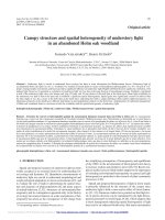
Figure 3. Map of the understory radiation for the Holm oak woodland studied. Maps represent indirect site factor (ISF, A and C) and direct site
factor (DSF, B and D) for either the shrub layer (A and B) or the herb layer (C and D). The map was based on 900 sampling points interpolated
by Krigging using spherical and exponential models for the semivariogram (see details and r
2
in Tab. VI). The two zones of the plot (tree- and
shrub-dominated zones) are indicated on the map. Distances shown in the axes are in m.
vegetation in many current Mediterranean ecosystems, where
abandoned woodlands and shrublands develop in the absence

of too frequent or intense perturbations towards still not well-
defined Holm oak forests [6].
Another distinctive feature of the understory light of the
studied Holm oak woodland was the long duration and high
intensity of sunflecks (Tab. II). Even though the fraction of
understory light provided by sunflecks (ca. 50%) was only
slightly lower than that for other temperate and tropical old
growth forests, their physiological implications could be very
different. Understory light in those old growth forests is very
scant (< 10% and even < 5% [4,8,53]), and sunflecks are short
and of moderate intensity so they are used in photosynthe-
sis very efficiently [35, 49], positively influencing survival and
performance of understory plants [10,36]. But sunflecks in the
understory of the studied Holm oak forest were very intense,
approaching full sunlight intensity in the open, and very long
(20–30 min vs. few s in mature, old growth forests [11]). These
two features make the photosynthetic exploitation of sunflecks
by understory plants very inefficient. In fact, long and intense
sunflecks can lead to severe photoinhibition, since the extent
of photoinhibition is proportional to the light dose [50].
The different spatial scales of light heterogeneity at each of
the two layers studied, with a range of the semivariogram of
5 m for the shrub layer and of 10–20 m for the herb layer, could
have important functional implications. The fine-grained light
heterogeneity at the shrub layer together with the large size
of individual plants indicates that this heterogeneity is mainly
exploited by different leaves of a given individual by means
of phenotypic plasticity. In contrast, the coarse-grained light
heterogeneity at the herb layer together with the small size of
individual plants indicates that this heterogeneity is exploited

by different micropopulations. Our study reveals that aban-
donment of traditional management of Holm oak woodlands
and the corresponding increase of shrub cover leads to a de-
crease in both the availability and the spatial heterogeneity of
understory light, but more research efforts are needed to under-
stand causes and consequences of changes in understory light
in Mediterranean forests if we are to predict and mitigate the
effects of global change on the regeneration and dynamics of
these forests.
4.2. Canopy structure and light interception: potentials
for indirect estimates of understory light
Quick and easy estimates of understory light are of great
potential for forest management since light determines many
functional processes and it is directly affected by most silvi-
cultural practices [3, 23, 46]. Since canopy structural features
determine light penetration, understory light can be estimated
by quantifying some of these features and both theoretical and
Understory light in an Holm oak woodland 759
Figure 4. Semivariograms for nine variables studied (see Tab. VI for more details). Values for the shrub (closed symbols) and herb (open
symbols) layers are given separately. Note that for the structural variables canopy height, number of stems and basal area no distinction
between layers was made and only one symbol is used.
empirical studies have been carried out in this direction for
more than four decades [1]. However, previous studies in trop-
ical forests have revealed a poor agreement between architec-
ture of dominant trees and understory light [5,31]. In our case,
despite the significant correlation of direct and indirect light
with vegetation height (Tab. VI), the regression models exam-
ined were not very robust. Although the forest canopy stud-
ied here is rather simple, only indirect radiation (ISF) could
be reasonably well estimated as a linear function of canopy

height, although only in the tree-dominated zone of the plot
(Tab. V). The value of canopy height as an estimator of under-
story light in forests similar to the one studied here relies on
the simplicity of its determination but not on the accuracy of
the estimations of understory light that can be obtained. The
incorporation of other canopy features (e.g. leaf angle distri-
bution, leaf and branch clustering) is likely to increase signifi-
cantly the accuracy of the estimation of understory light based
on canopy structure, but the advantages of this regression ap-
proach when compared with hemispherical photography itself
are likely to vanish due to the large efforts needed to determine
these features. Other variables such as basal area could also be
used for the estimation of understory light, but pilot studies are
needed to determine the best protocol and sampling scale and
density.
The inclusion of the three neighbor points situated immedi-
ately to the South of the target point significantly increased the
correlation of vegetation height and understory light (particu-
larly direct light, DSF), suggesting that pilot studies are nec-
essary to adjust the size and relative position of the area to be
sampled in each case. The size of this area and the agreement
between structural variables and understory light is specific for
each forest due to the varying influence of canopy height and
complexity, and latitude as shown elsewhere [14, 28, 31].
Acknowledgements: Special thanks are due to Libertad Gonzalez,
Daniela Brites, Silvia Matesanz, David Tena and David Sanchez for
support, to Itziar Rodriguez and Miguel Angel Zavala for facilitating
access to Holm oak data from the Spanish Forestry inventory, and to
Rebecca Montgomery for a critical revision of the manuscript. Finan-
cial support was provided by two grants of the Spanish Ministry for

Science and Technology (RASINV, CGL2004-04884-C02-02/BOS,
and PLASTOFOR, AGL2004-00536/FOR). BGA was supported by
a CSIC Introduction to Science fellowship.
REFERENCES
[1] Anderson M.C., Stand structure and light penetration. II. A theoret-
ical analysis, J. Appl. Ecol. 3 (1966) 41–54.
[2] Barbosa P., Wagner M.R., Introduction to forest and shade tree in-
sects, Academic Press, San Diego, 1989.
[3] Barnes B.B., Zak D.R., Denton S.R., Spurr S.H., Forest ecology,
John Wiley and Sons Inc., New York, 1998.
760 F. Valladares, B. Guzmán
[4] Beckage B., Clark J.S., Seedling survival and growth of three forest
tree species: the role of spatial heterogeneity, Ecol. 84 (2003) 1849–
1861.
[5] Bellow J.G., Nair P.K.R., Comparing common methods for assess-
ing understory light availability in shaded-perennial agroforestry
systems, Agric. For. Meteorol. 114 (2003) 197–211.
[6] Blondel J., Aronson J., Biology and wildlife of the Mediterranean
region, Oxford University Press, New York, 1999.
[7] Campbell G.S., Extinction coefficients for radiation in plant
canopies calculated using an ellipsoidal inclination angle distribu-
tion, Agric. For. Meteorol. 36 (1986) 317–321.
[8] Canham C.D., Denslow J.S., Platt W.J., Runkle J.R., Spies T.A.,
White P.S., Light regimes beneath closed canopies and tree-fall gaps
in temperate and tropical forests, Can. J. For. Res. 20 (1990) 620–
631.
[9] Canham C.D., Finzi A.C., Pacala S.W., Burbank D.H., Causes and
consequences of resource heterogeneity in forests – interspecific
variation in light transmission by canopy trees, Can. J. For. Res.
24 (1994) 337–349.

[10] Chazdon R.L., Sunflecks and their importance to forest understory
plants, Adv. Ecol. Res. 18 (1988) 1–63.
[11] Chazdon R.L., Pearcy R.W., The importance of sunflecks for forest
understory plants, BioSci. 41 (1991) 760–766.
[12] Chen J.M., Black T.A., Defining leaf area index for non-flat leaves,
Plant Cell Environ. 15 (1992) 421–429.
[13] Chen J.M., Black T.A., Adams R.S., Evaluation of hemispherical
photography for determining plant area index and geometry of a
forest stand, Agric. For. Meteorol. 56 (1991) 129–143.
[14] Clark D.B., Clark D.A., Rich P.M., Weiss S.B., Oberbauer S.F.,
Landscape-scale evaluation of understory light and canopy struc-
ture: methods and application in a neotropical lowland rain forest,
Can. J. For. Res. 26 (1996) 747–757.
[15] Ducrey M., Sylviculture des taillis de chêne vert. Pratiques tradi-
tionnelles et problématique des recherches récentes, Rev. For. Fr.
40 (1988) 302–313.
[16] Duncan R.P., Flood disturbance and the coexistence of species in a
lowland podocarp forest, south Westland, New Zealand, J. Ecol. 81
(1993) 403–416.
[17] Englund S.R., O’Brien J.J., Clark D.B., Evaluation of digital and
film hemispherical photography and spherical densiometry for mea-
suring forest light environments, Can. J. For. Res. 30 (2000) 1999–
2005.
[18] Ettema C.H., Wardle D.A., Spatial soil ecology, Trends Ecol. Evol.
17 (2002) 177–183.
[19] Ferres L., Biomasa, producción y mineralomasa del encinar de La
Castanya (Montseny), Ph.D. dissertation, Universidad Autónoma de
Barcelona, Spain, 1984.
[20] Gracia C., Response of the evergreen oak to the incident radiation
at the Montseny (Barcelona, Spain), Bull. Soc. Bot. Fr. 131 (1984)

595–597.
[21] Gracia C., Bellot J., Baeza J., Tello E., Sabate S., Roda F., A long-
term thinning experiment on a Quercus ilex L. forest: Main working
hypotheses and experimental design, in: International symposium
on experimental manipulations of biota and biogeochemical cycling
in ecosystems: approach, methodologies, findings, Copenhagen,
Denmark, 1992.
[22] Gratani L., Canopy structure, vertical radiation profile and
photosynthetic function in a Quercus ilex evergreen forest,
Photosynthetica 33 (1997) 139–149.
[23] Horn H.S., The adaptive geometry of trees, Princeton University
Press, Princeton, New Jersey, 1971.
[24] Instituto-Nacional-de-Meteorología, Calendario meteorológico
2003, Ministerio de Medio Ambiente, Madrid, 2003.
[25] Isaaks E.H., Srivastava R.M., An introduction to applied geostatis-
tics, Oxford University Press, New York, 1989.
[26] Jurena P.N., Archer S., Woody plant establishment and spatial het-
erogeneity in grasslands, Ecology 84 (2003) 907–919.
[27] Korning J., Thomsen K., A new method for measuring tree height
in tropical rain forest, J. Veg. Sci. 5 (1994) 139–140.
[28] Kuuluvainen T., Tree architectures adapted to efficient light utiliza-
tion: is there a basis for latitudinal gradients? Oikos 65 (1992) 275–
284.
[29] Legendre P., Forin M.J., Spatial pattern and ecological analysis,
Vegetatio, 80 (1989) 107–138.
[30] Miglioretti F., Contribution à l’étude de la production des taillis de
chêne vert en forêt de la Gardiole de Rians (Var), Ann. Sci. For. 44
(1987) 227–242.
[31] Montgomery R.A., Chazdon R., Forest structure, canopy architec-
ture, and light transmittance in tropical wet forests, Ecology 82

(2001) 2707–2718.
[32] Moran P.A.P., Notes on continuous stochastic phenomena,
Biometrika 37 (1950) 17–23.
[33] Nicotra A.B., Chazdon R.L., Iriarte S.V.B., Spatial heterogeneity
of light and woody seedling regeneration in tropical wet forests,
Ecology 80 (1999) 1908–1926.
[34] Nocentini S., Piusii P., Osservazioni priliminari sulla macchia del
Parco della Maremma, Inf. Bot. ital. 9 (1977) 174–184.
[35] Pearcy R.W., Sunflecks and photosynthesis in plant canopies, Ann.
Rev. Plant Physiol. Plant Mol. Biol. 41 (1990) 421–453.
[36] Pearcy R.W., Pfitsch W.A., The consequences of sunflecks for pho-
tosynthesis and growth of forest understory plants, in: Schulze
E D., Caldwell M.M. (Eds.), Ecophysiology of Photosynthesis,
Springer-Verlag, Heidelberg, 1994, pp. 343–359.
[37] Rich P.M., Characterizing plant canopies with hemispherical pho-
tographs, Remote Sens. Rev. 5 (1990) 13–29.
[38] Rich P.M., Clark D.B., Clark D.A., Oberbauer S.F., Long-term
study of solar radiation regimes in a tropical wet forest using quan-
tum sensors and hemispherical photography, Agric. For. Meteorol.
65 (1993) 107–127.
[39] Ross J., Sulev M., Sources of errors in measurements of PAR, Agric.
For. Meteorol. 100 (2000) 103.
[40] Roxburgh J.R., Kelly D., Uses and limitations of hemispherical pho-
tography for estimating forest light environments, N. Z. J. Ecol. 19
(1995) 213–217.
[41] Sabaté S., Sala A., Gracia C.A., Leaf traits and canopy organization,
in: Rodá F. et al. (Eds.), Ecology of Mediterranean evergreen oak
forests, Springer Verlag, Berlin, 1999, pp. 121–134.
[42] Sala A., Tenhunen J.D., Site-specific water relations and stomatal
response of Quercus ilex L. in a Mediterranean watershed, Tree

Physiol. 14 (1994) 601–617.
[43] Scarascia-Mugnozza G., Oswald H., Piussi P., Radoglou K., Forests
of the Mediterranean region: gaps in knowledge and research needs,
For. Ecol. Manage. 132 (2000) 97–109.
[44] Schnitzer S.A., Carson W.P., Treefall gaps and the maintenance of
species diversity in a tropical forest, Ecology 82 (2001) 913–919.
Understory light in an Holm oak woodland 761
[45] Serrada-Hierro R., Bravo-Fernández J.A., Roig-Gómez S.,
Brotación en encinas (Quercus ilex subsp. ballota) con edades
elevadas. Experiencias en el monte de Riofrío (Segovia), Investig.
Agrar. Sist. Recur. For. (2004) 127–141.
[46] Sonohat G., Balandier P., Ruchaud F., Predicting solar radiation
transmittance in the understory of even-aged coniferous stands in
temperate forests, Ann. For. Sci. 61 (2004) 629–641.
[47] Valladares F., Light and the evolution of leaf morphology and phys-
iology, Curr. Top. Plant Biol. 4 (2003) 47–61.
[48] Valladares F., Light heterogeneity and plants: from ecophysiology
to species coexistence and biodiversity, in: Esser K. et al. (Eds.),
Progress in Botany, Springer Verlag, Heidelberg, 2003, pp. 439–
471.
[49] Valladares F., Allen M.T., Pearcy R.W., Photosynthetic response to
dynamic light under field conditions in six tropical rainforest shrubs
occurring along a light gradient, Oecologia 111 (1997) 505–514.
[50] Valladares F., Pearcy R.W., The geometry of light interception by
shoots of Heteromeles arbutifolia: morphological and physiological
consequences for individual leaves, Oecologia 121 (1999) 171–182.
[51] Wagner H.H., Spatial covariance in plant communities: integrating
ordination, geostatistics, and variance testing, Ecology 84 (2003)
1045–1057.
[52] Weiss S.B., Rich P.M., Murphy D.D., Calvert W.H., Ehrlich P.R.,

Forest canopy structure at overwintering monarch butterfly sites –
Measurements with hemispherical photography, Conserv. Biol. 5
(1991) 165–175.
[53] Wiens J.A., Ecological heterogeneity: an ontogeny of concepts
and approaches, in: Hutchings M.J., John E.A., Stewart A.J.A.
(Eds.), The ecological consequences of environmental heterogene-
ity, Balckwell Science, Cambridge, 2000, pp. 9–31.
To access this journal online:
www.edpsciences.org/forest