Báo cáo lâm nghiệp: "Variables influencing cork thickness in spanish cork oak forests: A modelling approach" docx

Ann. For. Sci. 64 (2007) 301–312 301
c
 INRA, EDP Sciences, 2007
DOI: 10.1051/forest:2007007
Original article
Variables influencing cork thickness in spanish cork oak forests:
A modelling approach
Mariola S
´

-G
´

*
, Rafael C
,IsabelC
˜
, Gregorio M
Centro de Investigación Forestal, INIA, Ctra. de La Coruña, km 7,5, 28040 Madrid, Spain
(Received 27 March 2006; accepted 15 June 2006)
Abstract – In this study, we evaluate the influence of different variables on cork thickness in cork oak forests. For this purpose, first we fitted a multilevel
linear mixed model for predicting average cork thickness, and then identified the explanatory covariates by studying their possible correlation with
random effects. The model for predicting average cork thickness is described as a stochastic process, where a fixed, deterministic model, explains the
mean value, while unexplained residual variability is described and modelled by including random parameters acting at plot, tree, plot × cork harvest
and residual within-tree levels, considering the spatial covariance structure between trees within the same plot. Calibration is carried out by using
the best linear unbiased predictor (BLUP) theory. Different alternatives were tested to determine the optimum subsample size which was found to be
appropriate at four trees. Finally, the model was applied and its performance in the estimation of cork production was tested and compared with the
cork weight model traditionally used in Spain.
cork thickness / mixed model / calibration / Quercus suber L.
Résumé – Variables influençant l’épaisseur du liège dans les forêts de chênes-lièges espagnoles : une proposition de modélisation. Dans cette
étude, nous avons mesuré l’influence de diverses variables sur l’épaisseur du liège des forêts de chênes-lièges. Dans ce but nous avons d’abord appliqué

un modèle linéaire mixte pour prédire l’épaisseur moyenne du liège, et on a alors identifié les co-variables explicatives pour expliquer leur possible
corrélation avec des effets aléatoire. Le modèle prédisant l’épaisseur moyenne du liège peut être décrit comme un processus stochastique où un modèle
fixe et déterministe explique la valeur moyenne, tandis qu’une variabilité résiduelle inexpliquée est décrite et modélisée par l’inclusion de paramètres
aléatoires relevant de la parcelle, de l’arbre, de la récolte de liège par parcelle et aux niveaux résiduels des arbres prenant en compte la covariance de
la structure spatiale entre les arbres d’une même parcelle. Le calibrage a été réalisé en employant la théorie BLUP (Best linear unbiased predictor ou
Meilleur prédicteur linéaire non biaisé) On a essayé différentes options pour trouver la dimension optimale de l’échantillon et on a trouvé qu’il était
opportun d’utiliser quatre arbres par parcelles. Finalement le modèle a été appliqué pour calculer la production de liège et a été comparé avec le poids
de liège obtenu avec le modèle employé d’habitude en Espagne.
épaisseur du liège / modèle mixte / calibrage / Quercus suber L.
1. INTRODUCTION
Cork production constitutes a basic source of income in
cork oak stands prevailing in pre-coastal and coastal regions
of the Mediterranean Basin [11,31]. Spain is the second major
cork producing nation with 510 000 ha (23% of the world’s to-
tal) and an annual production of 110 000 t (32% of the world’s
total) [36]. Although the main use of these stands is cork pro-
duction, they are also efficiently exploited for other uses which
include hunting, cattle grazing, acorn production, firewood, or
biological and landscape diversity.
The management of these cork oak stands is oriented to-
wards cork production, in particular towards the maintenance
of cork quality. Cork quality depends on three main character-
istics: cork thickness, cork porosity and the presence of defects
such as insect galleries or wood inclusions which may appear
occasionally [31]. Cork thickness defines the usability and the
value of the cork for industrial purposes. Natural cork stoppers
* Corresponding author:
are the most valuable product and mainstay of the cork indus-
try. Cork planks with a thickness over 27 mm are suitable for
the production of stoppers, and the best yield is obtained with

a thickness of between 27 and 33 mm [18].
Despite its economic and industrial importance, research in
relation to cork thickness has been scarce. Vieira [45] studied
the influence of age and debarking height on cork thickness.
Montero and Vallejo [30] used data from 100 trees of differ-
ent sizes and stripped heights to study cork thickness varia-
tion along the bole. Cork thickness has seldom been modelled,
due to its great complexity and variability. González-Adrados
et al. [18] developed an equation for predicting total cork
thickness at debarking time where the independent variable
was cork thickness one year before stripping. A similar ap-
proach follows the cork thickness sub-model included in the
SUBER model [42], a management oriented growth and yield
model, developed in Portugal for open cork oak woodlands.
Among the numerous factors which appear to influence
cork thickness we might mention genetic variability [14], site
quality [29, 35], stand and single tree factors [5] as well as
Article published by EDP Sciences and available at or />302 M. Sánchez-González et al.
debarking factors [30, 45]. Due to the fact that many of these
factors are not easily controlled when modelling cork thick-
ness, stochastic models seem to provide the most suitable ap-
proach, especially during the first stages of modelling [25].
Cork thickness data are usually taken at each cork harvest
from trees growing in plots. This hierarchical structure favours
the use of a multi-level linear mixed approach. Mixed models
include a fixed functional part, common to the whole popula-
tion, and random components that allow us to divide and ex-
plain the different sources of stochastic variability which are
not explained by the fixed part of the model. Another advan-
tage of the mixed models is that they allow calibration of mod-

els for a specific location and period from a small additional
sample of observations. The mixed model approach was pro-
posed by Vázquez [44] for modelling single tree cork weight.
Empirical experience has shown that cork oak trees which
produce good cork quality, tend to maintain this standard in
successive strippings throughout their productive life [7]. In
the same way, it has been observed that there are productive
areas, where trees tend to have greater cork thickness, and that
these areas retain their productivity level throughout the cy-
cle. Finally, it is also possible to identify good and bad periods
for cork thickness, probably due to climatic effects [45]. All
these facts indicate that some unobservable tree factors (e.g.,
microsite or genetics), plot factors (ecological conditions or
silviculture) or period effects (climatic conditions) affect tree
cork thickness, even over long periods [29]. This allows us
to calibrate cork thickness models for present and future cork
harvests by introducing predicted stochastic effects into the
model which are specific to each source of variability.
The main objective of this study is to determine the vari-
ables which influence cork thickness by identifying the differ-
ent sources of variability detected in Spanish cork oak forests.
For this purpose we developed a multilevel linear mixed model
and evaluated the inclusion of ecological, stand and tree at-
tributes as fixed effects to explain detected non explained vari-
ability at different levels (plot, tree, harvest). Calibration of
the model from a small additional sample of observations was
proposed as a practical approach for model utilization, and its
accuracy in cork weight estimation was tested.
2. MATERIAL AND METHODS
2.1. Study area and data

The Natural Park of “Los Alcornocales” (Fig. 1), with an exten-
sion of 170 025 ha is one of the most important cork producing areas
in Spain and can be considered representative of Spanish cork oak
forests [38]. The area has a mild Mediterranean climate with cool hu-
mid winters and warm-dry summers; the mean annual temperature
is about 16−18
◦
C and the annual precipitation between 1000 and
1400 mm (depending on altitude). Precipitation is mainly concen-
trated between autumn and spring, originating a dry period in sum-
mer [10]. The soils are cambisols and luvisols (FAO) [12] which are
quite developed.
Data for this study were collected in 47 circular permanent plots
of 20 m radius established by the Forest Research Centre (CIFOR-
INIA) in the Natural Park. All plots were established between 1988
Figure 1. Distribution of Quercus suber L. in Spain and localization
of the studied region.
and 1993 in regularly stocked stands covering a wide range of age
and site conditions. In each plot, the first measurement was made at
plot installation coinciding with a cork harvest. The second inventory
was carried out at the time of the subsequent cork harvest (generally
after a nine year period).
The variables measured at each inventory were: perimeter at breast
height over and under cork, stripped height, cork weight and cork
thickness measured at the upper and lower ends of the three biggest
cork planks from each stripped tree. For each tree, average cork thick-
ness was calculated as the average of these six cork thickness mea-
surements. More recently, tree coordinates have been measured. In-
crement cores were not taken because they tend to be illegible [21],
so individual tree age is unknown. The age of the plot was estimated

using stem analysis data obtained near each plot in 2002 and the data
from the historic management records compiled from the Manage-
ment Plans and their subsequent Revisions [34]. Site index was calcu-
lated for each plot using the potential height growth model developed
by Sánchez-González et al. [38].
From this data set, 10 plots including 254 trees were selected as
a calibration data set. These plots were selected because measure-
ments were only taken at one cork harvest. The rest of the observa-
tions (coming from two repeated measurements taken on 795 trees
from 37 plots; totalling 1590 cork thickness observations) were used
as the fitting data set.
Descriptive statistics of cork characteristics for both data sets are
displayed in Table I.
2.2. Identification of variables influencing
cork thickness
The process of identification of variables influencing cork thick-
ness involved two stages. In the first stage, a multilevel linear mixed
model was fitted, in order to characterize the variability structure and
remove the effects of the spatial autocorrelation. In the second stage,
the explanatory covariates were identified by studying the correlation
between random effects and possible explanatory covariates.
Variables influencing cork thickness 303
Table I. Characterisation of the fitting and calibration data set.
Variable Mean Min Max STD CV (%)
Fitting data 1st harvest cb (mm) 25.59 11.63 57 6.03 23.58
w (kg) 21.7 4.5 141 14.97 68.98
sh (m) 1.79 0.77 5.4 0.61 34.25
Fitting data 2nd harvest cb (mm) 26.28 9 57.34 6.05 23.03
w (kg) 24.49 2.5 142.5 17.19 70.18
sh (m) 2.14 0.78 5.4 0.75 35.11

Calibration data cb (mm) 29.41 11.25 57.53 7.6 25.85
w (kg) 22.43 3 67 12.57 56.05
sh (m) 1.81 0.83 4.2 0.57 31.76
Min: Minimum; Max: maximum; STD: standard deviation; CV: coeffi-
cient of variation; cb: cork thickness (mm); w: tree cork weight (kg); sh:
stripped height (m).
2.2.1. Cork thickness modelling
The available fitting data set consists of a sample of cork thickness
measurements taken twice from trees located within different plots.
This hierarchical nested structure leads to lack of independence, since
a greater than average correlation is detected among observations
coming from the same tree, plot or cork harvest [16, 20].
In order to alleviate this, cork thickness is explained using a mul-
tilevel linear mixed model [4, 17, 41], including both fixed and ran-
dom components. In this model, systematic patterns of non explained
variability, detected between plots, between trees, and within a given
plot or within a given tree between different cork harvests were ac-
counted for by including random parameters, affecting the intercept
of the model, specific at those levels. A general expression for the
multilevel linear mixed model proposed, defined for the cork thick-
ness value (cb) measured on the j-th tree within the i-th plot, in the
k-th cork harvest, is:
cb
ijk
= x
ijk
β + u
i
+ v
ij

+ w
ik
+ e
ijk
(1)
where x
ijk
is 1 × p design vector containing covariates explaining the
response variable, β is the p × 1 vector of fixed parameters in the
model; u
i
,v
ij
,andw
ik
are random components specific for each plot,
tree and plot × cork harvest, realizations from univariate normal dis-
tributions with mean zero and variance σ
2
u
, σ
2
v
,andσ
2
w
respectively,
e
ijk
is a residual error term, with mean zero and variance σ

e
.Inclu-
sion of a common cork harvest effect was not considered, since cork
growth periods were different for different plots.
When fitting the framework, the available cork thickness out-
comes were N (1590), obtained from j trees ( j = 1toN
ij
, with N
ij
ranges from 11 to 42 trees per plot), growing within plot i (i = 1
to 37) in two different cork harvests (k = 1,2). For the complete data
set, the general expression of the model is [40]:
cb = Xβ + Zb + e(2)
where cb is the N × 1 vector containing the complete database of cork
thickness outcomes; X is a N × p design matrix with rows x
ijk
; β is
the p × 1 vector of fixed parameters in the model; Z is a N × qdesign
matrix, including zeroes and ones; b is a q × 1 vector of random com-
ponents, including in this analysis 795 tree components v
ij
,74plot×
cork harvest components w
ik
and 37 plot components u
i
;eisaN× 1
vector of residual tree within cork harvest terms.
Vector b is assumed to be distributed following a multivariate nor-
mal distribution with mean zero and variance matrix D,aq× qblock

diagonal matrix whose components are matrices D
u
, D
v
and D
w
.As
a first approach, we assumed independence between random compo-
nents specific to different sampling units (plot, tree, harvest) at the
same hierarchical level, so D
u
, D
v
and D
w
are diagonal matrices with
dimensions equalling the number of plots (37), trees (795) and plot ×
cork harvests (74) being considered in the analysis, and diagonal val-
ues of σ
2
u
, σ
2
v
and σ
2
w
. In subsequent steps different structures for D
u
and D

v
, were evaluated in terms of –2 times log likelihood statistic
by considering the spatial covariance between observations coming
from different plots or coming from different trees within the same
plot:
– Exponential covariance:
σ
12
= σ
2

exp

−d
12
ρ

(3)
– Gaussian covariance:
σ
12
= σ
2









exp








−

d
2
12

ρ
2

















(4)
– Power covariance:
σ
12
= σ
2

ρ
d
12

(5)
Where σ
12
indicates covariance between two observations, σ
2
indi-
cates the variance component (at plot or tree level), d
12
the distance
between the two trees or plots, and ρ is the correlation parameter.
Finally, vector e is distributed following a multivariate normal dis-
tribution with mean zero and variance matrix R, normally a N × N
diagonal matrix, with elements σ
2
e

.
The aim of the multilevel mixed analysis is to estimate the com-
ponents of β (fixed parameters of the model), D and R (variance
components), together with the prediction of the EBLUP (empirical
best linear unbiased predictor) for the random components associ-
ated with every plot, tree and plot × cork harvest (components of
vector b). Components were estimated using the restricted maximum
likelihood method in SAS procedure MIXED [28]. Level of signifi-
cance for variance components was analysed by means of the Wald
test, while level of significance for fixed parameters was tested using
Type III F-tests.
2.2.2. Explanatory covariates identification
In a first step, equation (1) was reduced to a basic model where
only the intercept µ and random components u
i
,v
ij
,w
ik
for the three
correlation levels considered (tree, plot and plot × cork harvest) were
taken into account. The basic multilevel mixed model expression for
cork thickness was:
cb
ijk
= µ + u
i
+ v
ij
+ w

ik
+ e
ijk
(6)
where µ is a fixed parameter defining the average cork thickness for
the studied population; u
i
,v
ij
,w
ik
and e
ijk
as defined in equation (1).
For this basic model, the predicted EBLUP’s for the random compo-
nents indicate systematic deviation from the population average cork
304 M. Sánchez-González et al.
thickness (µ) specific for the observations coming from the same plot,
tree and cork harvest, respectively.
This pattern of systematic variability can be explained by includ-
ing explanatory covariates (elements for vector x
ijk
in Eq. (1)) acting
at each of those specific levels. To identifiy those covariates which
best explain deviations, first we calculated the correlation coefficient
between EBLUP’s and different attributes at stand, ecological and
tree level. Only those variables showing significant correlation with
the EBLUP’s were evaluated for inclusion in model (6) as fixed
effects. Criteria for the final inclusion of a covariate in the model
were the level of significance for the parameters (fixed and random),

reduction in the value of the components of the variance-covariance
matrices, significant decrease for the statistic –2 times logarithm of
the likelihood function (−2LL) and rate of explained variability. The
variables evaluated were:
• At stand level
– Stand density: plot basal area under cork G
ha
(m
2
/ha); mean
squared diameter under cork d
g
(cm); number of trees per hectare
N
ha
(stems/ha); dominant diameter under cork d
dom
(cm), average
value for the 20% thickest trees within the plot.
– Other stand level covariates: canopy cover (%); age (years); site
index (m), calculated following Sánchez-González et al. [38].
• At tree level
– Tree-size: breast height diameter under cork d
uc
(cm); tree basal
area under cork g
uc
(m
2
); crown width cw (m).

– Relative tree dimension: diameter under cork divided by mean
squared diameter under cork d
uc
· d
−1
g
; diameter under cork di-
vided by maximum diameter under cork d
uc
· d
−1
max
; diameter un-
der cork divided by dominant diameter under cork d
uc
·d
−1
dom
; basal
area under cork divided by plot basal area under cork g
uc
· G
−1
;
basal area under cork divided by maximum basal area under cork
g
uc
· g
−1
max

; basal area under cork divided by dominant basal area
under cork g
uc
· g
−1
dom
; the relation between the basal area of the
ith tree and the total basal area divided by the number of trees per
hectare apb.
– Competition indices: basal area of trees larger than i tree BAL.
• Climatic attributes
Altitude (m); annual rainfall (mm); spring rainfall (mm); au-
tumn rainfall (mm); mean annual temperature (
◦
C); evapotranspi-
ration (mm); surplus (mm) sum of the difference between monthly
rainfall and evapotranspiration in months that potential evapotranspi-
ration is higher than monthly rainfall.
Climatic variables were obtained from the climatic models by
Sánchez Palomares et al. [39], developed using data from the weather
stations network of the National Institute of Meteorology and apply-
ing multiple linear regression methods with altitude, coordinates and
basin of the subject point as explanatory variables.
Summary statistics for the analysed variables are shown in
Table II.
2.3. Calibration
The main objective of the model is to detect the different sources
of variability in cork thickness. Together with this, the fitted model
can be used as a predictive tool for cork oak forest management.
Using the fixed effects part (x

ijk
β) of a mixed model, it is possible
to predict cork thickness in those locations where plot and tree ex-
planatory variables included in the model are measured. In this case,
we would obtain the fixed effects marginal prediction (i.e., value for
E[cb
ijk
]). Additionally, in a mixed model approach, it is possible to
calibrate the model by predicting the random component specific for
a new tree, plot or cork harvest, using a complementary sample of
cork thickness measured in that unit [27, 46]. Prediction of the ran-
dom components is carried out using empirical best linear unbiased
predictors (EBLUP) [40]:
ˆ
b =
ˆ
D
ˆ
Z
T

ˆ
R +
ˆ
Z
ˆ
D
ˆ
Z
T


−1
ˆ
e (7)
where
ˆ
b is a vector including predicted random components for the
new sampled units;
ˆ
D,
ˆ
Z and
ˆ
R are matrices including the predicted
components for D, Z and R, defined for the additional sample; ê is
a vector whose components are the values for the marginal uncondi-
tional residuals for the new sample (difference between the observed
and the predicted cork thickness using the fixed effects marginal
model). Inclusion of vector
ˆ
b will allow us to obtain a random effects
conditional prediction (i.e. E[cb
ijk
|
ˆ
b]). To solve
ˆ
b from equation (7),
a SAS program was developed using IML language.
The accuracy of the calibration was evaluated using the data from

the ten plots in the calibration data set comparing different alterna-
tives of subsample size of cork thickness measurements in the plots
(1, 2, 4, 6, 8 and 10 trees randomly selected). For each plot and
subsample size, 100 random realizations were performed, each time
including different trees in the calibration subsample. The statistics
used in the comparison were: modelling efficiency (MEF) and root
mean square error (RMSE) estimated as the mean value after 100 re-
alizations.
MEF = 1 −
n

i=1

y
i
− ˆy
i

2
n

i=1

y
i
−
_
y

2

(8)
RMSE =


y
i
− ˆy
i

2
n − 1
(9)
where y
i
,ˆy
i
and y represents observed, predicted and average value
for variable y; n represents the number of observations.
3. RESULTS
3.1. Cork thickness modelling
The results obtained after fitting the basic model in equa-
tion (6), considering simple variance structures for matrices
D and R, are included in the first column of Table III. The
comparison of different spatial covariance structures for D re-
vealed that the best results were obtained by considering a sim-
ple variance structure for matrix D
u
(no spatial correlation be-
tween plots) and a Gaussian spatial covariance structure for
matrix D

v
, indicating a pattern of spatial correlation between
random tree components for the same plot (Tab. III, columns
2−4). All parameters, both for the basic and spatial models,
were significant at the 0.01 level. Figure 2 shows the evolu-
tion of the pattern of spatial correlation between two trees as
a function of distance, indicating that cork thickness shows
Variables influencing cork thickness 305
Table II. Characterisation of variables evaluated as possible explanatory covariates.
Variable Mean Min Max STD CV (%)
Stand attributes G
ha
(m
2
ha
−1
) 17.73 8.38 27.05 4.49 25.34
N
ha
(stems ha
−1
) 195.29 87.00 334.00 62.82 32.17
d
g
(cm) 35.21 24.33 56.86 6.35 18.03
Site index (m) 10.16 6.00 14.00 2.92 28.74
Canopy cover (%) 15.86 8.60 26.62 4.67 29.44
d
dom
(cm) 42.01 29.48 79.29 8.29 19.72

Age (years) 98.30 53.00 177.00 31.61 32.16
Climatic attributes Altitude (m) 588 180.00 820.00 182.88 31.09
Annual rainfall (mm) 1257 1070.00 1391.00 81.54 6.49
Spring rainfall (mm) 330 279.00 363.00 21.93 6.64
Autumn rainfall (mm) 310 266.00 338.00 18.81 6.06
Annual Temperature (
◦
C) 16.00 15.00 18.00 0.67 4.13
Evapotranpiration (mm) 826.00 792.00 879.00 25.39 3.07
Surplus (mm) 884.00 688.00 1013.00 84.49 9.56
Tree attributes d
uc
(cm) 31.12 14.01 61.43 7.13 22.92
g
uc
(m
2
) 0.08 0.02 0.30 0.04 47.36
Crown diameter (m) 3.05 0.50 7.10 0.93 30.66
d
uc
·d
−1
g
0.93 0.42 1.55 0.18 19.37
d
uc
·d
−1
max

0.89 0.17 2.41 0.34 38.51
d
uc
·d
−1
dom
0.59 0.14 1.00 0.20 34.18
g
uc
·G
−1
0.39 0.02 1.00 0.24 60.79
g
uc
·g
−1
max
0.80 0.41 1.34 0.15 18.45
g
uc
·g
−1
dom
0.67 0.17 1.79 0.24 36.26
apb 45.14 6.64 133.34 22.63 50.13
BAL (m
2
/ha) 11.57 0.00 26.82 5.79 50.09
Min: Minimum; Max: maximum; STD: standard deviation; CV: coefficient of variation; G
ha

: plot basal area under cork; N
ha
: number of trees per ha;
d
g
: mean square diameter under cork; d
dom
: dominant diameter under cork; d
uc
: diameter at breast height under cork; g
uc
: tree basal area under cork;
d
max
: maximum diameter under cork of the plot; G: plot basal area under cork; g
max
: maximum basal area under cork; g
dom
: dominant basal area under
cork; apb: area proportional to tree basal area; BAL: mean basal area of the trees larger than ith tree where d
j
> d
i
.
Table III. Comparison of fitting statistics and estimated variance components of the basic and spatial models.
Basic linear mixed model Exponential spatial structure model Gaussian spatial structure model Power spatial structure model
µ 25.7731 25.7724 25.7621 25.7724
ρ 1.6805 2.0107 0.5516
σ
2

u
(tree) 19.4756 19.5968 19.4642 19.5970
σ
2
v
(plot) 5.9588 5.6889 5.8933 5.6896
σ
2
w
(plot × 3.9412 3.9429 3.6430 3.9449
cork harvest)
σ
2
e
(error) 7.5337 7.5321 7.5235 7.5319
−2LL 9332.6 9329.9 9323.6 9324.9
µ: Fixed parameter defining the average cork thickness for the studied population; ρ: correlation parameter; σ
2
: variance terms; −2LL: −2 times
logarithmic of likelihood.
306 M. Sánchez-González et al.
Figure 2. Spatial correlogram for tree random effect, comparing
Gaussian (solid line) with power and exponential (dashed lines) co-
variance structures (overlapped).
spatial correlation, at tree level, up to a distance of 5 m. The
spatial correlograms corresponding to the power and exponen-
tial covariance structures are overlapped. Under the proposed
Gaussian spatial structure, the components of the variance ma-
trix for the observations V would be:
– Variance for a single observation:

σ
2
u
+ σ
2
v
+ σ
2
w
+ σ
2
e
– Covariance between two observations taken in the same
inventory, from two trees in the same plot separated a dis-
tance d
12
:
σ
2
u
+ σ
2
w
+ σ
2
v









exp








−

d
2
12

ρ
2

















– Covariance between two observations taken in different in-
ventories from the same tree:
σ
2
u
+ σ
2
v
– Covariance between two observations taken in different in-
ventories from different trees in the same plot, separated a
distance d
12
:
σ
2
u
+ σ
2
v









exp








−

d
2
12

ρ
2

















The highest level of variability (53%) is associated with tree
effects, while the between cork harvest random effect for plots
accounted for the lowest level (10%) of the total non explained
variability. Plot level effects explain 16% of the variability
while the remaining 21% is associated with residual (tree ×
cork harvest) effects.
The mean variance value obtained for the e
ijk
conditional
residual terms after fitting the basic model was computed
for each different class of explanatory variables and plotted
against them. No pattern of non-constant variance in the resid-
uals (heteroscedasticity) was detected, indicating that the se-
lected simple structure for matrix R is adequate. The plot of
e
ijk
against predicted values (not shown) displays an increas-
ing trend, indicating the need to identify explanatory covari-
ates which are dealt with in the next section.
Table IV. Correlation coefficients of plot random effect and stand and
ecological covariates.
Covariates Pearson’s coefficient P value
Stand attributes

Basal area –0.1383 0.4402
Density 0.0770 0.6504
Mean square diameter –0.1211 0.4753
Site index –0.2692 0.1071
Canopy cover –0.1823 0.2777
Dominant diameter 0.0955 0.9553
Age 0.2651 0.1128
Ecological attributes
Altitude 0.1403 0.9343
Annual rainfall –0.1620 0.3379
Spring rainfall –0.1382 0.4146
Autumn rainfall –0.1381 0.415
Annual temperature –0.0099 0.9536
Evapotranspiration –0.0217 0.8986
Surplus –0.1450 0.3918
To test the behaviour in σ
2
v
the variance for EBLUP’s v
ij
was computed per categorical class for the different stand at-
tributes considered in Table II. We detected a pattern (not
shown) of reduction in variance associated with increasing
classes of canopy cover, basal area and mean squared diam-
eter and decreasing classes of stand density. This indicates
that within plot tree variability in cork thickness is larger in
younger phases of stand development, tending towards homo-
geneity in mature states. After evaluating various alternatives,
the following model for tree level variance depending on mean
squared diameter was proposed:

σ
2
v
= 0.0566 d
2
g
− 4.8556 d
g
+ 114.04 (10)
3.2. Identification of explanatory covariates
The EBLUP’s for random parameters u
i
,v
ij
and w
ik
were
expanded over different covariates. Tables IV and V show the
correlation coefficients between random components and pos-
sible explanatory covariates as well as their transformations.
None of the stand or climatic attributes evaluated were identi-
fied as significantly correlated with random plot components.
In order to evaluate possible trends, charts of the predicted
EBLUP’s u
i
for random plot effect against the stand and eco-
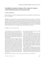
logical variables were also assessed. From this graphical anal-
ysis, a slight positive trend with age was detected (r = 0.26,
p = 0.10; Fig. 3), indicating that older stands tend to have
thicker cork than younger ones. No significant relation was

identified between plot-level EBLUP’s u
i
and climatic vari-
ables (Fig. 4). Regarding tree attributes, initial tree diameter
and section area were significantly correlated with predicted
EBLUP’s for v
ij
at the 0.05 level, while several competition
Variables influencing cork thickness 307
Table V . Correlation coefficients of tree random effect and tree co-
variates.
Covariates Pearson’s coefficient P value
d
uc
0.0737 0.0377
g
uc
0.0703 0.0362
cw 0.0642 0.0782
d
uc
·d
−1
g
0.1038 0.0034
d
uc
·d
−1
max

0.0633 0.0747
d
uc
·d
−1
dom
0.0954 0.0071
g
uc
·G
−1
0.1089 0.0021
g
uc
·g
−1
max
0.0606 0.0875
g
uc
·g
−1
dom
0.0172 0.0041
apb 0.0737 0.0371
BAL –0.0891 0.0129
d
uc
: Diameter at breast height under cork; g
uc

: tree basal area under cork;
cw: crown width; d
g
: mean square diameter under cork; d
max
:plotmax-
imum diameter under cork; d
dom
: dominant diameter under cork; G: plot
basal area under cork; g
max
: maximum basal area under cork; g
dom
: domi-
nant basal area under cork; apb: area proportional to tree basal area; BAL:
mean basal area of the trees larger than ith tree where d
j
> d
i
.
Figure 3. Random plot effect in relation to plot age.
indices (d
uc
· d
−1
g
,d
uc
· d
−1

dom
,g
uc
· G
−1
,g
uc
· g
−1
dom
, apb) were sig-
nificantly correlated at 0.01 level.
Only those covariates significantly correlated with random
components were evaluated for inclusion in the model in a
linear form. Several models including different subsets of ex-
planatory variables were evaluated in terms of −2 log likeli-
hood ratio tests. Although the inclusion of tree level attributes
lead to significant likelihood improvements, it was finally de-
cided that none of the models which considered explanatory
covariates would be used because, at best, the percentage of
explained variability was less than 2%.
3.3. Calibration
As none of the explanatory covariates were identified as
significant and useful in explaining cork thickness variability,
calibration was proposed as an alternative approach to obtain
estimates for cork thickness. Figure 5 shows the results of the
calibration carried out in the ten plots of the calibration data
set, comparing different sizes of sample for calibrating cork
thickness. These additional measurements were used to pre-
dict both random plot and plot × cork harvest components,

which were then added to the model.
Calibration tends to be more efficient as subsample size in-
creases, although only small differences exist between a four-
tree sample and a larger one. Calibration using four trees lead
to modelling efficiencies (at plot level) between 0.15 and 0.60
(except for plot 57, not shown in the figure, where calibration
does not improve the use of the average population model).
The root mean square error obtained through a four-tree cali-
bration ranges from 4.75 to 8.33 mm (except for plot 53, where
RMSE is over 10 mm).
Case study: application of the calibration approach
to estimate cork production
In the study area, cork weight at tree level has traditionally
been estimated using the model proposed by Montero [29],
where cork weight is given by the following expression:
w = 13.44 · sh · cbh (11)
Where w is cork weight just after debarking (kg), sh is stripped
height (m) and cbh is circumference at breast height under
bark (m).
In this study we propose the use of the developed cork
thickness model to predict cork weight, using the following
expression:
w = cb · sh · cbh · cork density (12)
Where w, sh and cbh are as previously stated; cb is predicted
cork thickness (in mm) and cork density is referred to as the
relation between cork weight and volume, which has been cal-
culated for the area at 420 kg/m
3
.
Data from the ten calibration plots were used to estimate

cork weight using both expressions (11) and (12). Table VI
shows the relative error (13) in estimating cork weight at-
tained using the Montero [29] approach (11), or using expres-
sion (12), calibrating cork thickness with different subsample
sizes.
Relative error (%) = 100

ˆy − y

y
(13)
Where y and y represents estimated (from Eq. (11) or Eq. (12))
and observed plot cork weight respectively. Using the present
model, calibration using cork thickness data from only four
additional trees, leads to a relative error under 10% in eight
of the ten plots analysed, giving slightly better results than the
previous model, except for plots 53−55.
The proposed calibration approach also allows the estima-
tion of cork weight from trees with a mean cork thickness
greater than 27 mm, which is considered the limit value for
the stopper industry. This was done by estimating cork weight
308 M. Sánchez-González et al.
Figure 4. Random plot effect in relation to main climatic attributes.
at tree level which involved, along with the predicted random
plot and plot × cork harvest components, a stochastic tree level
component defined by a random realization from a normal dis-
tribution with mean zero and common plot variance given by
equation (10). For each plot we have computed 100 Monte
Carlo simulations, randomly assigning a stochastic component
for each tree in each simulation, and computing cork produc-

tion destined for the stopper industry as the average value for
those 100 realizations. Figure 6 shows the relation between
observed and predicted cork weight per plot for the stopper
industry. The relative errors obtained in predicting cork for
the stopper industry ranges from 2−15% (except for plot 21,
where the model predicted 145 kg, while the observed cork
weight for the stopper industry was only 48 kg).
4. DISCUSSION
4.1. Identification of variables influencing
cork thickness
In this study, we evaluate the influence of different vari-
ables on cork thickness in cork oak forests. For this purpose,
first we fitted a multilevel linear mixed model for predicting
average cork thickness, including random parameters acting
at plot, tree, plot × cork harvest and residual within-tree lev-
els, and considering spatial covariance structure between trees
within the same plot. In a second step the explanatory co-
variates were identified by studying their possible correlation
with random effects. The mixed model approach was proposed
by Vázquez [44] for modelling cork weight prediction and
for modelling the yield of other non-timber products, such as
stone pine cones [3] or cowberry production [23].
The largest part of non-explained variability (53%) is as-
sociated with tree effect. Tree size, given by breast height di-
ameter or section, and relative tree dimension indices, have a
positive correlation with random tree effect. This positive cor-
relation with size and competition indexes, might be related
to the fact that in Mediterranean ecosystems water use (avail-
ability and temporal variation) is more efficient in larger indi-
viduals [24, 26]. Vázquez [44] obtained a similar result when

modelling cork weight prediction.
The results obtained indicate that unobservable tree fac-
tors, which remain constant from one cork harvest period to
the next, exert some influence over cork thickness. These fac-
tors can be related to microsite or genetics. It is known that
cork quality variability is high even under identical site con-
ditions [7, 14, 18, 45], so results suggest a close relationship
between cork thickness and genetic aspects. The small corre-
lation distance (< 5 m) detected among tree random compo-
nents from the same plot may confirm the strong dependence
of cork thickness on genetic factors, as trees within a short dis-
tance of each other would more than likely belong to the same
parent tree or stump sprout. The predicted EBLUP’s for the
random tree component, specific to each tree, might be con-
sidered indices for selecting trees with the highest cork pro-
duction once plot or period effects have been accounted for,
indicating the utility of mixed models in genetic improvement
programs [22].
Sixteen percent of the non-explained variability is related to
between-plot variability. When representing random plot ef-
fect vs. age (Fig. 3) a slight trend can be identified as cork
thickness is greater in older stands. A similar trend was de-
tected by Costa et al. [8] in their analysis of cork growth vari-
ability, in which they reported a slight trend of increasing cork
increments with tree diameter. In the other hand, Vieira [45]
Variables influencing cork thickness 309
Figure 5. Modelling efficiency (MEF) and root mean square error (RMSE) for cork thickness estimation in calibration data set (10 plots), as a
function of the number of trees used in calibration.
Table VI. Relative error in estimating cork weight using the model by Montero (1987) and the model proposed in the present work comparing
different subsample size for calibration.

PLOT N w Montero (1987)
Calibration sample size
1 tree 2 trees 4 tress 6 trees 8 trees 10 trees
21 39 540 76.57% 35.35% 29.36% 23.77% 22.05% 19.69% 18.43%
53 19 633 –2.76% –15.14% –11.63% –9.31% –6.20% –5.35% –5.06%
54 13 450 –4.52% –15.15% –12.58% –8.14% –5.77% –4.29% –3.71%
55 14 354 –5.66% –17.80% –15.19% –11.34% –9.69% –8.59% –7.99%
56 18 642 7.33% –6.92% –4.40% –1.79% 0.21% 1.27% 2.09%
57 12 422 17.87% –3.00% –2.13% –2.08% –2.42% –1.72% –1.39%
58 33 821 4.41% –7.87% –4.93% 1.14% 3.36% 5.54% 6.73%
59 26 532 12.25% –2.62% –0.66% 4.01% 6.89% 6.97% 9.02%
60 40 683 7.89% –7.77% –3.55% 0.48% 0.75% 1.93% 2.83%
61 40 623 18.70% 1.25% 2.92% 5.89% 8.05% 8.20% 8.22%
All plots 254 5698 13.16% –3.81% –1.98% 0.76% 2.28% 2.99% 3.58%
w: Cork weight (kg/plot); N: number of trees per plot.
310 M. Sánchez-González et al.
Figure 6. Observed versus predicted (using calibration from four trees per plot) cork weight for stopper industry in calibration plots.
and Figueroa [15] detected through a graphical assessment,
a significant decrease in cork thickness after tenth debarking.
Plots we analysed were mainly between 65 and 135 years old,
so most of the plots have still not reached the 10th debark-
ing rotation. This could explain the fact that no significant de-
creasing correlation between plot age and random plot effect
has been detected in our work.
We found no correlation between cork thickness and stand
density attributes. This result is in accordance with Cañellas
et al. [5] and Torres et al. [43], who reported that density does
not influence cork thickness, at least for the range of density
values in the data set used for those studies.
Cork thickness is related to site conditions, as stated

by Ferreira et al. [14], Corona et al. [7] and Montero
and Cañellas [32]. Despite this, the site index proposed by
Sánchez-González et al. [38] is not significantly correlated
with random plot effects. Traditional site indices, using domi-
nant height as an indicator of timber productivity, have shown
their validity in predicting growth and timber yield in Mediter-
ranean species [1,3,33], but do not work so well when used to
estimate other productions, such as pine nuts, cork or resin,
which in Mediterranean ecosystems could constitute more
than 50% of the total annual biomass produced [2]. More
exhaustive site indices which include ecological factors are
needed for the species. Therefore, this line of research should
be considered a priority for future studies.
This lack of relationship between cork thickness and den-
sity or site index is directly related to the high variability found
in trees growing in the same neighbourhood and confirms the
result that most of the cork thickness variability is associated
with tree effect. In that sense, it would be important to find an
indicator which permits the evaluation of cork thickness at tree
level prior to the establishment of the stand or in very young
plantations. For this purpose, isotopic fingerprints of soils and
vegetations have been used to find possible relationships be-
tween stable isotope measurements at natural abundance lev-
els and the quality of the standing tree mass in Pinus pinaster
and Pinus sylvestris plantations [13], as well as in multiple
regression models to predict the site index variation in Pinus
radiata stands [19]. In future research, it would be interesting
to try this technique in order to evaluate future cork thickness
at tree level or to use soil isotopic signatures in process models
to predict cork thickness.

Previous studies concerning the influence of climate on
cork growth have concluded that the main climatic factors are:
summer drought [6], summer temperatures [6], spring precipi-
tation [37] and autumn-winter precipitations [6,8,9,37]. How-
ever, in the present study, climatic attributes were not found
to be correlated with cork thickness. The result for the pre-
cipitation parameters can be explained by the fact that in the
study area, the annual precipitation varies between 1000 and
1400 mm (depending on altitude), whereas in the aforemen-
tioned studies, the areas under analysis receive a mean an-
nual precipitation of around 600 mm. We must also take into
account that those studies related annual cork increments to
annual or monthly values of the climatic factors whilst our
study used mean values for climatic parameters at each de-
barking period. Possible effects may have been lost through
using mean values.
The between-cork-harvest variability at plot level accounts
for 10% of total variability, indicating differences between
growth periods, at least at plot level, almost certainly related
to long-term climatic effects like drought, such as that suffered
in Spain between 1993 and 1995. The between-cork-harvest
residual variance at tree level accounts for 21% of the total
non-explained variability. This could be related to abnormal
variations in debarking intensity, either because of prior de-
barking damages or as a result of years of conditions that make
cork extraction more difficult, such as hot windy days or seri-
ous attacks of Lymantria dispar (among others) [31].
4.2. Calibration
None of the models which considered explanatory covari-
ates were used because, at best the percentage of explained

variability, it was less than 2%. Nevertheless, by identifying
Variables influencing cork thickness 311
the different sources of variability it is possible to calibrate the
model for new locations using a small amount of cork thick-
ness data (obtained using a cork calliper) from each plot.
When additional measurements from four trees per plot
were used for calibration, the modelling efficiency was over
30% in 7 of the 10 calibration plots analysed, indicating a
significant improvement over using an average cork thickness
value for the entire region. In any case, considering that plot
and plot × cork harvest levels jointly explain 26% of non-
explained variability in the fitting data set, it is unlikely that
the results obtained would be improved by including a larger
number of trees in the calibration subsample. With respect to
RMSE, calibration reduces it by more than 2 mm in 8 of the
calibration plots when compared to the original deviation from
the population average. These values are deemed as accept-
able, taking into account the large within-plot variability in
cork thickness detected. In general, calibration at plot level
tends to be more effective in those plots where average cork
thickness is largely deviated with respect to the average cork
thickness for the population.
The proposed four trees calibration approach could be use-
ful in predicting cork weight, obtaining better predictions than
Montero’s model [29]. The main advantage of the proposed
approach compared to previously developed models is that to-
gether with cork weight, it is possible to estimate cork thick-
ness, which is the variable that most affects cork value. By
using Monte Carlo simulations to assign random components
for each tree within the plot it is possible to use the calibration

approach to classify total cork production at plot level. For ex-
ample, trees with a mean cork thickness of less than 27 mm
would not be useful for the stopper industry.
5. CONCLUSIONS
The model developed help us to improve our knowledge of
cork thickness variability, identifying sources of non explained
variability and allowing us to identify further factors (at tree,
stand or period level), which need to be analysed for future
improvements to the model.
The model confirms the slight relationship between silvi-
culture and cork thickness, and the probable dependence of
this variable on unobservable site factors not related with av-
erage climatic conditions.
Large variability in cork thickness is associated with unob-
servable tree attributes, probably to do with genetics or mi-
crosite rather than social status.
Prediction of random components using a small sample of
additional measurements converts the proposed model into a
useful tool for predicting cork thickness and weight, allowing
us to classify the cork with respect to its final use in the cork
industry. In that sense, calibration measuring cork thickness in
four trees per plot seems an interesting and low cost approach
when compared to previously developed models.
Acknowledgements: The research was partially supported by a
grant to the corresponding author from the CIFOR-INIA. The au-
thors wish to thank E. Torres for providing plot and tree coordinates.
We also wish to thank the two anonymous reviewers for their helpful
comments and suggestions.
REFERENCES
[1] Bravo-Oviedo A., del Río M., Montero G., Site index curves and

growth model for Mediterranean maritime pine (Pinus pinaster
Ait.) in Spain, For. Ecol. Manage. 201 (2004) 187−197.
[2] Cabanettes A., Rapp M., Biomasse, minéralomasse et productivité
d’un écosystème à pins pignons (Pinus pinea L.) du littoral méditer-
ranéen. III. Croissance, Acta Oecol. Plant. 2 (1981) 121−136.
[3] Calama R., Modelo interregional de selvicultura para Pinus pinea
L. Aproximación mediante funciones con componentes aleatorio,
Ph.D. thesis, Universidad Politécnica de Madrid, 2004.
[4] Calama R., Montero G., Multilevel linear mixed model for tree
diameter increment in stone pine (Pinus pinea): a calibrating ap-
proach, Silva Fenn. 39 (2005) 37−54.
[5] Ca˜nellas I., Bachiller A., Montero G., Influencia de la densidad
de la masa en la producción de corcho en alcornocales adehesa-
dos de Extremadura, Actas del Congreso de Ordenación y Gestión
Sostenible de Montes, Santiago de Compostela, 4−9deOctubrede
1999, Ponencias y Resúmenes de Comunicaciones, Tomo I, 2000,
pp. 449−456.
[6] Caritat A., Gurierrez E., Molinas M., Influence of weather on cork-
ring width, Tree physiol. 20 (2000), 893−900.
[7] Corona P., Dettori S., Filigheddu M.R., Maetzke F., Scotti R., Site
quality evaluation by classification tree: an application to cork qual-
ity in Sardinia, Eur. J. For. Res. 124 (2005) 37−46.
[8] Costa A., Pereira H., Oliveira A., Variability of radial growth in
cork oak mature trees under cork production, For. Ecol. Manage.
175 (2003) 239−246.
[9] Costa A., Pereira H., Oliveira A., Influence of climate on the sea-
sonality of radial growth of cork oak during a cork production cycle,
Ann. For. Sci. 59 (2002) 429−437.
[10] De Benito Ontañón N., Cork oak stands in Cortes de la Frontera,
Proceedings of the IUFRO Meeting Mediterranean Silviculture with

emphasis in Quercus suber, Pinus pi nea and Eucalyptus sp., 2000.
[11] Falcao A.O., Borges J.G., Designing decision support tools for
Mediterranean forest ecosystems management: case study, Ann.
For. Sci. 62 (2005) 751−760.
[12] FAO, World Reference Base for Soil Resources, World Soil
Resources Reports, 84, Rome, 1998.
[13] Fernández I., González-Prieto A.J., Cabaneiro A., C-isotopic finger-
prints of Pinus pinaster Ait. and Pinus sylvestris L. wood related to
the quality of standing tree mass in forests from NW Spain, Rapid
Commun. Mass Spectrom. 19 (2005) 3199−3206.
[14] Ferreira A., Lopes F., Pereira H., Caractérisation de la croissance et
de la qualité du liège dans une région de production, Ann. For. Sci.
57 (2000) 187−193.
[15] Figueroa P., Alcornocales e Industria Corchera, Conferencia sobre
alcornocales, E.T.S.I. Montes, Madrid, 1957.
[16] Fox J.C., Ades P.K., Bi H., Stochastic structure and individual-tree
growth models, For. Ecol. Manage.154 (2001) 261−276.
[17] Goldstein H., Multilevel Statistical Models, 2nd. ed., Arnold
Publishers, London, 1995.
[18] González Adrados J.R., González Hernández R., Calvo Haro R., La
predicción del calibre de corcho al final del turno y su aplicación
al muestreo de la producción, Investig. Agrar., Sist. Recur. For. 9
(2000) 363−373.
[19] González-Prieto S.F., Villar M.C. Soil organic N dynamics and
stand quality in Pi nus radiata pinewoods of the temperate humid
region, Soil Biol. Biochem. 35 (2003) 1395−1404.
312 M. Sánchez-González et al.
[20] Gregoire T.G., Generalized error structure for forestry yield models,
For. Sci. 33 (1987) 423−444.
[21] Gourlay I.D., Pereira H., The effect of bark stripping on wood pro-

duction in cork-oak (Quercus suber L.) and problems of growth
ring definition, in: Pereira H. (Ed.), Proceedings of the European
Conference on Cork Oak and Cork, Centro de Estudos Florestais,
Lisboa, 1998, pp. 99−107.
[22] Henderson C.R., Kempthorne O., Searle S.R., Von Krosing C.N.,
Estimation of environmental and genetic trends from records sub-
ject to culling, Biometrics 15 (1959) 192−218.
[23] Ihalainen M., Salo K., Pukkala T., Empirical prediction models for
Vaccinium myrtillus and V. vitis-idaea berry yields in North Karelia,
Finland, Silva Fenn. 37 (2003) 95−108.
[24] Koechlin B., Rambal S., Debussche M., Rôle des arbres, pionniers
sur la teneur en eau du sol en surface de friches de la región méditer-
ranéenne, Acta Oecol. 7 (1986) 177−190.
[25] Kyrikiadis P.C., Journel A.G., Geostatistical space-time models: a
review, Math. Geol. 31 (1999) 651−684.
[26] Landsac A.R., Zaballos J.P., Martin A., Seasonal water poten-
tial changes and proline accumulation in Mediterranean shrubland
species, Vegetatio, 113 (1994) 141−154.
[27] Lappi J., Bailey R.L., A height prediction model with random stands
and tree parameters: an alternative to traditional site index methods,
For. Sci. 34 (1988) 907−927.
[28] Littell R.C., Milliken A.G., Stroup W.W., Wolfinger R.D., SAS sys-
tem for mixed models, SAS Institute Inc., Cary, NC, 1996, 633 p.
[29] Montero G., Modelos para cuantificar la producción de corcho en
alcornocales (Quercus suber L.) en función de la calidad de estación
y los tratamientos selvícolas, Ph.D. thesis, INIA, Madrid, 1987,
277 p.
[30] Montero G., Vallejo R., Variación del calibre de corcho medido
a distintas alturas, Investig. Agrar., Sist. Recur. For. 2 (1992)
181−188.

[31] Montero G., Cañellas I., Manual de forestación del alcornoque
(Quercus suber L.), MAPA-INIA, 1999.
[32] Montero G., Cañellas I., Selvicultura de los alcornocales en España,
Silva Lusitana 11 (2003) 1−19.
[33] Montero G., Cañellas I., Ruiz-Peinado R., Growth and yield mod-
els for Pinus halepensis Mill., Investig. Agrar. Sis. Recur. For. 10
(2001) 179−202.
[34] Montes F., Sánchez M., Del Rio M., Cañellas I., Using historic
management records to characterize the effects of management on
the structural diversity of forests, For. Ecol. Manage. 207 (2005)
279−293.
[35] Montoya J.M., Los alcornocales, S.E.A., Madrid, 1988.
[36] Natural Cork Quality Council Industry statistics, Natural Cork
Quality Council, Sebastopol, CA, USA, 1999, Online at
.
[37] Oliveira G., Martins-Loução M.A., Correira O. The relative impor-
tance of cork harvesting and climate fore stem radial growth of
Quer cus s uber L., Ann. For. Sci. 59 (2002) 439−443.
[38] Sánchez-González M., Tomé M., Montero G., Modelling height and
diameter growth of dominant cork oak trees in Spain, Ann. For. Sci.
62 (2005) 1−11.
[39] Sánchez-Palomares O., Sánchez Serrano F., Carretero Carrero
M.P., Modelos y cartografía de estimaciones climáticas termoplu-
viométricas para la España peninsular INIA, col. Fuera de Serie,
Madrid, 1999.
[40] Searle S.L., Casella G., McCulloch C.E., Variance components,
John Wiley & sons, Inc, New York, 1992, 501 p.
[41] Singer J.D., Using SAS PROC MIXED to fit multilevel models,
hierarchical models, and individual growth models, J. Educational
Behavioural Statistics 23, (1998) 323−355.

[42] Tomé M., Coelho M. B., Almeida A., Lopes, F., O mod-
elo SUBER. Estrutura e equações utilizadas, Relatórios técnico-
científicos do GIMREF n
◦
2/2001, Centro de Estudos Florestais,
Instituto Superior de Agronomia, Lisboa, 2001.
[43] Torres E., Montero G., Suarez M.A., Relación entre la densidad
de la mas y la producción de corcho en montes alcornocales del
sur de España, in: Puertas F., Rivas M. (Eds), II Congreso Forestal
Nacional, Tomo IV, 1997, pp. 529−534.
[44] Vazquez F.J., Modelos preditivos de produçao de cortiça e detecçao
precoce da qualidade, Ph.D. thesis, ISA, Lisboa, 2002
[45] Vieira Natividade J., Subericultura, D.G.F.P., Lisboa, 1950.
[46] Vonesh E.F., Chinchilli V.M., Linear and nonlinear models for the
analysis of repeated measurements, Marcel Dekker, Inc., New York,
1997.