Báo cáo lâm nghiệp: "A growth model for Pinus radiata D. Don stands in north-western Spain" doc

Ann. For. Sci. 64 (2007) 453–465 Available online at:
c
 INRA, EDP Sciences, 2007 www.afs-journal.org
DOI: 10.1051/forest:2007023
Original article
AgrowthmodelforPinus radiata D. Don stands
in north-western Spain
Fernando C-D
a
*
, Ulises D

´
-A
b
, Juan Gabriel Á    -G
´

b
a
Departamento de Ingeniería Agraria, Universidad de León. Escuela Superior y Técnica de Ingeniería Agraria, Avenida de Astorga,
24400 Ponferrada, Spain
b
Departamento de Ingeniería Agroforestal, Universidad de Santiago de Compostela, Escuela Politécnica Superior, Campus universitario,
27002 Lugo, Spain
(Received 15 September 2006; accepted 20 December 2006)
Abstract – A dynamic whole-stand growth model for radiata pine (Pinus radiata D. Don) stands in north-western Spain is presented. In this model,
the initial stand conditions at any point in time are defined by three state variables (number of trees per hectare, stand basal area and dominant height),
and are used to estimate total or merchantable stand volume for a given projection age. The model uses three transition functions derived with the
generalized algebraic difference approach (GADA) to project the corresponding stand state variables at any particular time. These equations were fitted
using the base-age-invariant dummy variables method. In addition, the model incorporates a function for predicting initial stand basal area, which can

be used to establish the starting point for the simulation. Once the state variables are known for a specific moment, a distribution function is used to
estimate the number of trees in each diameter class by recovering the parameters of the Weibull function, using the moments of first and second order
of the distribution. By using a generalized height-diameter function to estimate the height of the average tree in each diameter class, combined with a
taper function that uses the above predicted diameter and height, it is then possible to estimate total or merchantable stand volume.
whole-stand growth model / radiata pine plantations / generalized algebraic difference approach / basal area disaggregation / Galicia
Résumé – Un modèle de croissance pour des peuplements de Pinus radiata D. Don du nord ouest de l’Espagne. Un modèle dynamique de
croissance de peuplement est présenté pour Pinus radiata D. dans le nord ouest de l’Espagne. Dans ce modèle, les conditions initiales du peuplement
en tout point et temps sont définies par trois variables d’état (nombre d’arbres à l’hectare, surface terrière et hauteur dominante) et sont utilisées pour
estimer le volume total ou marchand du peuplement pour un âge donné. Le modèle utilise trois fonctions de transition dérivées avec une approche par
différence algébrique généralisée (GADA) pour projeter les variables d’état correspondantes du peuplement à n’importe quel moment. Ces équations
ont été ajustées en utilisant la méthode des variables indicatrices indépendantes de l’âge. En plus, le modèle incorpore une fonction de prédiction de
la surface terrière initiale du peuplement qui peut être utilisée pour établir le point de départ de la simulation. Une fois que les variables d’état sont
connues à un instant donné, une fonction de distribution est utilisée pour estimer le nombre d’arbres dans chaque classe de diamètre en récupérant les
paramètres de la fonction de Weibull, en utilisant les moments de premier et de second ordre de la distribution. En utilisant une fonction généralisée
hauteur-diamètre pour estimer la hauteur de l’arbre moyen de chaque classe de diamètre, combinée avec une fonction qui utilise la prédiction précédente
du diamètre et de la hauteur, il est alors possible d’estimer le volume total ou marchand du peuplement.
modèle de croissance de peuplement / plantations de Pinus radiata / approche par différence algébrique généralisée / désagrégation de la surface
terrière / Galice
1. INTRODUCTION
A managed forest is a dynamic biological system that is
continuously changing as a result of natural processes and
in response to specific silvicultural activities. Forest manage-
ment decisions are based on information about current and
likely future forest conditions. Consequently, it is often nec-
essary to predict the changes in the system using growth and
yield models, which estimate forest dynamics over time. Such
models have been widely used in forest management because
they allow updating of inventories, prediction of future yields,
and exploration of management alternatives, thus providing in-
* Corresponding author:

formation for decision-making in sustainable forest manage-
ment [42, 98]. Forest growth models can be categorised ac-
cording to their level of mechanistic detail in empirical growth
and yield models and process-based models [9]. Although em-
pirical growth models do little to elucidate the mechanisms
of tree or stand growth, they are more widely used as prac-
tical tools in forest management, perhaps because of their
simplicity.
According to Vanclay [99], Gadow and Hui [47] and Davis
et al. [36], empirical growth and yield models can be grouped
into three types of models that represent a broad contin-
uum: whole-stand models, size-class models and individual-
tree models. The most appropriate type of model depends
on the intended use, the stand characteristics, the resources
Article published by EDP Sciences and available at or />454 F. Castedo-Dorado et al.
available and the projection length [17, 51, 98]. These factors
also determine which data are required and the resolution of
the estimates. Individual-tree growth models provide more de-
tailed information than is available from other modelling ap-
proaches [50,51], and usually perform better than whole-stand
models for short term projections [17]. For forest management
planning, however, standard forest inventories do not usually
provide sufficiently reliable estimates for initializing the tree-
level starting conditions required by individual-tree models.
Furthermore, over-parameterization of the functions may of-
ten limit accuracy and precision of quantitative predictions.
Moreover, aggregated outputs from these types of models are
required for decision-making, resulting in a projection of a
simple state description through complicated functions.
At least for even-aged, single-species stands, whole-

stand models are an attractive alternative, which directly
project information that is easily obtained from inventory
data [48,51,98]. In addition, model errors in inventory data
may be magnified by individual-tree models but remain less al-
tered by simpler models such as whole-stand models. In sum-
mary, whole-stand models may be preferable for plantation
management planning applications because they represent a
good compromise between generality and accuracy of the es-
timates [46,51].
Whole-stand models require few details for growth sim-
ulation, but provide rather limited information about the
future stand (in some cases only stand volume) [98, 99].
Considering that forest management decisions require more
detailed information about stand structure and volume, as
classified by merchantable products, whole-stand models can
be disaggregated mathematically using a diameter distribu-
tion function, which may be combined with a generalized
height-diameter equation and with a taper function to esti-
mate commercial volumes that depend on certain specified
log dimensions. Similar methodologies have been used by
Cao et al. [20], Burk and Burkhart [14], Clutter et al. [32],
Knoebel et al. [59], Zarnoch et al. [104], Uribe [97], Río [85],
Mabvurira et al. [68], Kotze [60], Trincado et al. [96], and
Diéguez-Aranda et al. [40] in the development of forest growth
models, mainly for plantations.
Radiatapine(Pinus radiata D. Don) is well represented in
the north of Spain, especially in the Basque Country and Gali-
cia. According to the Third National Forest Inventory, radi-
ata pine stands occupy a total surface area of approximately
90 000 ha in Galicia [102], with a current rate of planting of

about 6 000 ha per year [1]. The wide distribution and the high
growth rate of the species have also made it very important in
the forestry industry in northern Spain, with an annual harvest
volume of around 1 600 000 m
3
[70]. More than one third of
this timber comes from Galicia. Nevertheless, to date, the only
whole-stand growth model for the species in this region is a
yield table developed by Sánchez et al. [88]. This model pro-
vides limited information about the forest stand and does not
reflect accurately the evolution under different stand density
conditions.
The objective of the present study was to develop a
management-oriented dynamic whole-stand model for simu-
lating the growth of radiata pine plantations in Galicia. The
model is constituted by the following interconnected submod-
els: a site quality system, an equation for reduction in tree
number, a stand basal area growth system, and a disaggrega-
tion system composed of a diameter distribution function, a
generalized height-diameter relationship and a total and mer-
chantable volume equation. All of the submodels were devel-
oped in the present study, except the site quality system and the
height-diameter relationship, which have already been pub-
lished [23, 39].
2. MATERIAL AND METHODS
2.1. Data
The data used to develop the model were obtained from three dif-
ferent sources. Initially, in the winter of 1995 the Sustainable Forest
Management Unit of the University of Santiago de Compostela es-
tablished a network of 223 plots in pure radiata pine plantations in

Galicia. The plots were located throughout the area of distribution
of this species in the study region, and were subjectively selected to
represent the existing range of ages, stand densities and sites. The
plot size ranged from 625 to 1200 m
2
, depending on stand density,
to achieve a minimum of 30 trees per plot. All the trees in each sam-
ple plot were labelled with a number. The diameter at breast height
(1.3 m above ground level) of each tree was measured twice (mea-
surements at right angles to each other), with callipers – to the nearest
0.1 cm – and the arithmetic mean of the two measurements was cal-
culated. Total height was measured to the nearest 0.1 m with a digital
hypsometer in a randomized sample of 30 trees, and in an additional
sample including the dominant trees (the proportion of the 100 thick-
est trees per hectare, depending on plot size). Descriptive variables of
each tree were also recorded, e.g., if they were alive or dead.
After examination of the data for evidence of plots installed in
extremely poor site conditions, and taking into account that some
plots had disappeared because of forest fires or clear-cutting, a subset
of 155 of the initially established plots was re-measured in the win-
ter of 1998. Following similar criteria, a subset of 46 of the twice-
measured plots were measured again in the winter of 2004. Between
each of the three inventories, 22 plots were lightly or moderately
thinned once from below. These plots were also re-measured imme-
diately before and after thinning operations. The first source of data
comprises the inventories carried out in 1995, 1998, and 2004 and on
the date of the thinning operations.
In addition, data from the first and second measurements of two
thinning trials installed in a 12-year old stand of radiata pine were
also used. Each thinning trial consisted of 12 plots of 900 m

2
,in
which four thinning regimes were evaluated on three different oc-
casions. The four thinning treatments considered were: an unthinned
control, a light thinning from below, a moderate thinning from be-
low, and a selection thinning (selection of crop trees and extraction
of their competitors). The plots were thinned immediately after plot
establishment in 2003 and were re-measured three years later. The
second source of data corresponds to the first and second inventories
of these thinning trials.
For the fist two sources of data, the following stand variables were
calculated for each plot and inventory: age (t), number of trees per
hectare (N), stand basal area (G), and dominant height (H,definedas
the mean height of the 100 thickest trees per hectare). Only live trees
were included in the calculations for stand basal area and number of
A growth model for Pinus radiata D. Don stands in north-western Spain 455
Table I. Summarised data corresponding to the sample of plots and trees used for model development.
Variable 1st inventory (247 plots) 2nd inventory (179 plots) 3rd inventory (46 plots)
Mean Max. Min. S.D. Mean Max. Min. S.D. Mean Max. Min. S.D.
t (years) 21.6 38 5 8.3 24.0 41 8 8.7 30.5 47 20 7.5
H(m) 19.0 32.5 5.9 5.4 21.2 34.0 11.0 4.9 26.6 35.2 17.8 4.2
G (m
2
ha
−1
) 31.1 87.1 5.2 11.4 35.2 63.0 16.5 9.6 44.1 64.0 28.4 7.9
N(stems ha
−1
) 964.8 2048 200 459.2 895.8 1968 191.7 436.0 744.6 1488 280 311.7
421 trees

d (cm) 28.2 60.0 5.1 12.8
h (m) 20.4 36.5 4.2 6.5
v (m
3
) 0.759 3.56 0.006 0.769
t = stand age; H = dominant height; G = stand basal area; N = number of stems per hectare; d = diameter at breast height over bark; h = total tree
height; v = total tree volume over bark above stump level.
trees per hectare. In addition, data on the number of trees per hectare
and stand basal area removed in thinning operations were available.
Apart from these inventories, two dominant trees were destruc-
tively sampled at 82 locations in the winters of 1996 and 1997. These
trees were selected as the first two dominant trees found outside the
plots but in the same plantations within ± 5% of the mean diame-
ter at 1.3 m above ground level and mean height of the dominant
trees. Total bole length of felled trees was measured to the nearest
0.01 m. The logs were cut at 1 to 2.5 m intervals; the number of
rings was counted at each cross-sectional point, and then converted
to age above stump height. As cross-section lengths do not coincide
with periodic height growth, we adjusted height-age data from stem
analysis to account for this bias using Carmean’s method [21] and
the modification proposed by Newberry [75] for the topmost section
of the tree. Additionally, 257 non-dominant trees were felled outside
the 82 locations to ensure a representative distribution by diameter
and height classes for taper function development. Log volumes were
calculated by Smalian’s formula. The top of the tree was considered
as a cone. Tree volume above stump height was aggregated from the
corresponding log volumes and the volume of the top of the tree. The
third source of data corresponds to the 421 trees felled.
Summary statistics, including the mean, minimum, maximum, and
standard deviation of the stand and tree variables used in model de-

velopment are given in Table I.
2.2. Model structure
The model is based on the state-space approach [50], which as-
sumes that the behaviour of any system evolving in time can be es-
timated by describing its current state, usually through a finite list of
state variables (state vector), and a rate of change of state as a func-
tion of the current variables.
The state of a system at any given time may be roughly defined as
the information needed to determine the behaviour of the system from
that time on; i.e., given the current state, the future does not depend
on the past [50]. Silvicultural treatments, such as thinning, cause an
instantaneous change in the state variables of the stand, and therefore
the system must estimate the trajectories starting from the new state
after thinning. The requirements for an adequate state description are
that the change in each of the state variables should be determined,
to an appropriate degree of approximation, by the current state. In
addition, it should be possible to estimate other variables of interest
from the current values of the state variables through the so-called
output functions [50, 51].
In selecting the state variables, the principle of parsimony must be
taken into account [17, 46, 50, 99]: the model should be the simplest
one that describes the biological phenomena and remains consistent
with the structure and function of the actual biological system [73].
For unthinned stands, a two dimensional vector including dominant
height and stand basal area as explanatory variables may be sufficient
to describe the state of the stand at a given time [80]. Nevertheless,
in situations covering a wide range of silvicultural regimes, the inclu-
sion of an additional variable such as the number of trees per unit area
is necessary [4, 50–52]. A fourth state variable representing relative
site occupancy or canopy closure may improve predictions in some

instances (especially when heavy thinning and pruning has been un-
dertaken), at the cost of added complexity in model usage [49–51].
Transition functions are used to predict the growth by updat-
ing the state variables, and they must possess some obvious prop-
erties [50]: (i) consistency, which implies no change for zero elapsed
time; (ii) path-invariance, where the result of projecting the state first
from t
0
to t
1
, and then from t
1
to t
2
, must be the same as that of the
one-step projection from t
0
to t
2
; and (iii) causality, in that a change
in the state can only be affected by inputs within the relevant time
interval. Transition functions generated by integration of differential
equations (or summation of difference equations when using discrete
time) satisfy these conditions and allow computation of the future
state trajectory.
Considering that we are dealing with single-species stands derived
from plantations in which different management regimes have been
carried out, three state variables (dominant height, number of trees
per hectare and stand basal area) are needed to define the stand con-
ditions at any point in time. These state variables are used to estimate

stand volume, classified by commercial classes. The model uses three
transition functions of the corresponding state variables, which are
used to project the future stand state. Once the state variables are
known for a given time, the model is disaggregated mathematically
by use of a diameter distribution function, which is combined with
a generalized height-diameter equation and with a taper function to
estimate total and merchantable stand volumes.
The following sections describe how each of the three transition
functions and the disaggregation system were developed.
456 F. Castedo-Dorado et al.
2.3. Development and fitting of transition functions
2.3.1. Model development
Fulfilment of the above mentioned properties for the transition
functions depends on both the construction method and the mathe-
matical function used to develop the model. Most of these properties
can be achieved by using techniques for dynamic equation derivation
known in forestry as the Algebraic Difference Approach (ADA) [6] or
its generalization (GADA) [28]. Dynamic equations have the general
form (omitting the vector of model parameters) of Y = f
(
t, t
0
, Y
0
)
,
where Y is the value of the function at age t,andY
0
is the reference
variable defined as the value of the function at age t

0
. The ADA essen-
tially involves replacing a base-model site-specific parameter with its
initial-condition solution. The GADA allows expansion of the base
equations according to various theories about growth characteristics
(e.g., asymptote, growth rate), thereby allowing more than one pa-
rameter to be site-specific and allowing the derivation of more flexi-
ble dynamic equations (see [24–26]).
The first step in the ADA or GADA is to select a base equation
and identify in it any desired number of site-specific parameters (only
one parameter in ADA). An explicit definition of how the site spe-
cific parameters change across different sites must be provided by
replacing the parameters with explicit functions of X (one unobserv-
able independent variable that describes site productivity as a sum-
mary of management regimes, soil conditions, and ecological and cli-
matic factors) and new parameters. In this way, the initially selected
two-dimensional base equation
(
Y = f
(
t
))
expands into an explicit
three dimensional site equation
(
Y = f
(
t, X
))
describing both cross

sectional and longitudinal changes with two independent variables t
and X.SinceX cannot be reliably measured or even functionally de-
fined, the final step involves the substitution of X by equivalent initial
conditions t
0
and Y
0
(
Y = f
(
t, t
0
, Y
0
))
so that the model can be im-
plicitly defined and practically useful [25,28].
The ADA or GADA can be applied in modelling the growth
of any site dependent variable involving the use of unobservable
variables substituted by the self-referencing concept [77] of model
definition [27], such as dominant height, number of trees per unit
area or stand basal area.
2.3.2. Model fitting
The individual trends represented in dominant height, number of
trees per hectare and stand basal area data of the plots can be mod-
elled by considering that individuals’ responses all follow a sim-
ilar functional form with parameters that vary among individuals
(local parameters) and parameters that are common for all individ-
uals (global parameters). In practice both base-age specific (BAS)
and base-age invariant (BAI) methods can be used. The assumption

behind the BAS methods, which use selected data (e.g., heights at
the given base age) as site-specific constants, is that the data mea-
surements simultaneously do and do not contain measurement and
environmental errors (on the left- and right-hand sides of the model,
respectively) (e.g., [35, 74], which is clearly untenable [6]. The as-
sumption behind the BAI methods, which estimate site-specific ef-
fects, is that the data measurements always contain measurement and
environmental errors (both on the left- and right-hand sides of the
model) that must be modelled [26]. From among the different BAI
parameter estimation techniques available, we estimated the random
site-specific effects simultaneously with the fixed effects by using the
dummy variables method described by Cieszewski et al. [29]. In this
method the initial conditions are specified as identical for all the mea-
surements belonging to the same individual (tree or plot). The initial
age can be, within limits, arbitrarily selected; however, age zero is not
allowed. The variable corresponding to the initial age is then simul-
taneously estimated for each individual along with all of the global
model parameters during the fitting process. The dummy variables
method recognizes that each measurement is made with error and,
therefore, it does not force the model through any given measure-
ment. Instead, the curve is fitted to the observed individual trends in
the data. With this method all the data can be used, and there is no
need to make any arbitrary choice regarding measurement intervals.
The dummy variables method was programmed using the SAS/ETS

MODEL procedure [91].
In the general formulation of the dynamic equations, the error
terms e
ij
are assumed to be independent and identically distributed

with zero mean. Nevertheless, because of the longitudinal nature of
the data sets used for model fitting, correlation between the residuals
within the same individual may be expected, in which case an appro-
priate fitting technique should be used (see [105]). This problem may
be especially important in the development of the dominant height
dynamic model on the basis of data from stem analysis, because of
the number of measurements corresponding to the same tree. Never-
theless, in the construction of the dynamic equations for reduction in
tree number and for basal area growth, which involve the use of data
from the first and second inventory of 179 plots and from the third
inventory of 46 of these plots, respectively, the maximum number of
possible time correlations among residuals is practically inexistent,
and therefore the problem of autocorrelated errors can be ignored in
the fitting process.
2.4. Transition function for dominant height growth
The site quality system, which combines compatible site index
and dominant height growth models in one common equation, was
developed by Diéguez-Aranda et al. [40]. The authors (op. cit.)
took into consideration the following desirable attributes for domi-
nant height growth equations: polymorphism, sigmoid growth pat-
tern with an inflexion point, horizontal asymptote at old ages, logical
behaviour (height should be zero at age zero and equal to site in-
dex at the reference age; the curve should never decrease), theoretical
basis or interpretation of model parameters derived by analytically
tractable algebraic operations, base-age invariance, and path invari-
ance [6, 25, 26,28]. Possession of multiple asymptotes was also con-
sidered a desirable attribute [25].
With these criteria in mind, Diéguez-Aranda et al. [39] exam-
ined different base models and tested several variants for each
one, in which both one and two parameters were considered to be

site-specific. The GADA formulation derived from the Bertalanffy–
Richards model by considering the asymptote and the initial pat-
tern parameters as related to site productivity (Eq. (9) in the original
publication) resulted in the best compromise between graphical and
statistical considerations and produced the most adequate site index
curves.
2.5. Transition function for reduction in tree number
A dynamic equation was developed for predicting the reduction
in tree number due to density-dependent mortality, which is mainly
A growth model for Pinus radiata D. Don stands in north-western Spain 457
caused by competition for light, water and soil nutrients within a
stand [79]. According to Clutter et al. [31], most mortality analyses
are based on the values of age and number of trees per hectare at the
beginning and at the end of the period involved. Therefore, the model
was constructed using data from the plots measured more than one
time.
Although many functions have been used to model empirical mor-
tality equations, only biologically-based functions derived from dif-
ferential equations include the set of properties that are essential in a
mortality model [31, 101]: consistency, path invariance and asymp-
totic limit of stocking approaching zero as old ages are reached.
Moreover, for even-aged stands it is usually assumed that in-growth
is negligible [101].
In the present study, the equation for estimating reduction in tree
number was developed on the basis of a differential function in which
the relative rate of change in the number of stems is proportional to
an exponential function of age:
dN/dt
N
= αN

β
δ
t
(1)
where N is the number of trees per hectare at age t,andα, β and δ are
the model parameters.
This function was selected by Álvarez González et al. [3] to de-
velop an equation in difference form for estimating reduction in stem
number by using data from the first two inventories of the network of
permanent plots described in the Data section. In the present study, a
new dynamic equation developed by use of the ADA was fitted with
the BAI dummy variables method to data from all the plot inventories
available.
2.6. Transition function for stand basal area growth
The GADA was used to develop a function for projecting stand
basal area. This requires having an initial value for stand basal area at
a given age, which may generally be obtained from a common forest
inventory where diameter at breast height is measured. If the initial
stand basal area is not known, it must be estimated from other stand
variables by use of an initialization equation. The stand basal area
growth system is therefore composed of two sub-modules: one for
stand basal area initialization and another for projection.
In the development of the stand basal area projection function,
efforts were focused on six dynamic equations derived by applying
the GADA to the base equations of Korf (cited in Lundqvist [67]),
Hossfeld [54] and Bertalanffy-Richards [10, 11, 84]). For each base
equation one (the scale parameter) and two parameters were consid-
ered to be site specific (see [8]).
The initialization function was developed on the basis of the cor-
responding base growth function from which the dynamic model that

provided the best results on projection was derived. Because stand
basal area at any specific point in time depends on stand age and
other stand variables (theoretically the productive capacity of the site
and any other measure of stand density), it was necessary to relate
the site-specific parameters of the base function to these variables to
achieve good estimates.
To ensure compatibility between the projection and initialization
functions, the former must be developed on the basis of the same base
growth function used for initialization. In addition, the site-specific
parameters must be related to stand variables that do not vary over
time (e.g., site index), whereas the remaining parameters must be
shared by both functions. If any of these requirements is not reached,
compatibility is not ensured.
The projection function was fitted with data from all the plots
measured more than one time, whereas the initialization sub-module
was only fitted with data from 98 inventories, corresponding to ages
younger than 15 years, and assuming that if projections based on
ages older than this threshold are required, the initial stand basal area
should be obtained directly from inventory data.
2.7. Disaggregation system
2.7.1. Diameter distribution
Many parametric density functions have been used to describe
the diameter distribution of a stand (e.g., Charlier, Normal, Beta,
Gamma, Johnson SB, Weibull). Among these, the Weibull function
has been the most frequently used for describing the diameter dis-
tribution of even-aged stands because of its flexibility and simplicity
(e.g., [7, 18, 58, 68,95]).
Expression of the Weibull density function is as follows:
f (x) =


c
b

x − a
b

c−1
e
−
(
x−a
b
)
c
(2)
where x is the random variable, a the location parameter that defines
the origin of the function, b the scale parameter, and c the shape pa-
rameter that controls the skewness.
The Weibull parameters can be obtained by different methodolo-
gies, which can be classified into two groups: parameter estimation
and parameter recovery [56,96,98]. Several researchers have reported
that the parameter recovery approach provides better results than pa-
rameter estimation, even in long-term projections [12, 20, 83, 95].
According to Parresol [78], the parameter recovery method is gen-
erally better than the parameter prediction method for projecting fu-
ture distribution parameters, because diameter frequency distribution
characteristics, such as mean diameter and diameter variance, can
be projected with more confidence than the distribution parameters
themselves.
The parameter recovery approach relates stand variables to per-

centiles [19] or moments [15,76] of the diameter distribution, which
are subsequently used to recover the Weibull parameters. The mo-
ments method is the only method that directly warrants that the sum
of the disaggregated basal area obtained by the Weibull function
equals the stand basal area provided by an explicit growth function of
this variable, resulting in numeric compatibility [44,56–58,71,95]. It
was therefore the method selected for the present study.
In the moments method, the parameters of the Weibull function
are recovered from the first three order moments of the diameter dis-
tribution (i.e., mean, variance and skewness coefficient, respectively).
Alternatively, the location parameter (a) may be set to zero. The use
of this condition restricts the parameters of the Weibull function to
two, thus making it easier to model, and providing similar results
to the three-parameter Weibull, at least for even-aged, single-species
stands [2, 68, 69]. Thus, to recover parameters b and c the following
expressions were used:
var =
¯
d
2
Γ
2

1 +
1
c


Γ


1 +
2
c

− Γ
2

1 +
1
c

(3)
b =
¯
d
Γ

1 +
1
c
 (4)
458 F. Castedo-Dorado et al.
where
¯
d is the arithmetic mean diameter of the observed distribution,
var is its variance, and Γ is the Gamma function.
Once the mean and the variance of the diameter distribution are
known at any specific time, and taking into account that Equation (4)
only depends on parameter c, the latter can be obtained using iterative
procedures. Parameter b can then be calculated directly from Equa-

tion (5). Considering that the disaggregation system is developed for
inclusion in a whole-stand growth model, only the arithmetic mean
diameter requires to be modelled, because the variance can be directly
obtained from the arithmetic and the quadratic mean diameters (d
g
)
by the relationship var = d
2
g
−
¯
d
2
.
The arithmetic mean diameter may be estimated at any point in
time by the following expression [44], which ensures that predictions
of
¯
d are lower than d
g
for the ordinary range of stand conditions:
¯
d = d
g
− e
Xβ
(5)
where X is a vector of explanatory variables (e.g., dominant height,
number of treesper hectare,age )that characterizethestateofthe
stand at a specific time and must be obtained from any of the func-

tions of the stand growth model, and β is a vector of parameters to
be estimated. This procedure has been widely used in diameter distri-
bution modelling in which the parameter recovery approach is used
(e.g., [14, 20, 59]).
A diagram of the disaggregation system including all the compo-
nents proposed in the present study is reported by Diéguez-Aranda
et al. [40].
2.7.2. Height estimation for diameter classes
Once the diameter distribution is known, it is necessary to esti-
mate the height of the average tree in each diameter class. A local
height-diameter (h-d) relationship may be used for this purpose; nev-
ertheless, the h-d relationship varies from stand to stand, and even
within the same stand this relationship is not constant over time [34].
Therefore, a single curve cannot be used to estimate all the possible
relationships that can be found within a forest. To minimise the level
of variance, h-d relationships can be improved by taking into account
stand variables that introduce the dynamics of each stand into the
model (e.g., [34, 66, 93]).
The generalized h-d model used in the present study was devel-
oped by Castedo et al. [23] on the basis of the Schnute [92] function,
which is one of the most flexible and versatile functions available
for modelling this relationship [65]. Castedo et al. [23] modified the
original Schnute function by forcing it (i) to pass through the point
(0, 1.3) to prevent negative height estimates for small trees, and (ii) to
predict the dominant height of the stand (H
0
) when the diameter at
breast height of the subject tree (d) equals the dominant diameter of
the stand (D
0

) (see Eq. (3) in the original publication).
2.7.3. Total and merchantable volume estimation
Once the diameter and height of the average tree in each diameter
class are estimated, the total tree volume can be calculated directly by
use of a volume equation. If volume prediction to any merchantable
limit is required, two methods are commonly applied. One is to de-
velop volume ratio equations that predict merchantable volume as a
percentage of total tree volume (e.g., [16]). The other is to define an
equation that describes stem taper (e.g., [62]); integration of the taper
equation from the ground to any height will provide an estimate of
the merchantable volume to that height. Merchantable volume equa-
tions obtained from taper functions are preferred nowadays, perhaps
because they allow easy estimation of diameter at a given height.
Ideally, a volume estimation system should be compatible, i.e.,
the volume computed by integration of the taper equation from the
ground to the top of the tree should be equal to that calculated by a
total volume equation [30,37]. The total volume equation is preferred
when classification of the products by merchantable sizes is not re-
quired, thereby simplifying the calculations and making the method
more suitable for practical purposes. An up-to-date review of com-
patible volume systems is provided by Diéguez-Aranda et al. [41].
Data on diameter at different heights and total stem volume from
421 destructively sampled trees were used for fitting a compatible
system. To correct the inherent autocorrelation of the hierarchical
data used, and taking into account that observations within a tree
were not equally distributed, the error term was expanded by using
an autoregressive continuous model, which can be applied to irregu-
larly spaced, unbalanced data [105]. To account for k-order autocor-
relation, the CAR(x) error structure expands the error terms in the
following way:

e
ij
=

k=x
k=1
I
k
ρ
h
ij
−h
ij−k
k
e
ij−k
+ ε
ij
(6)
where e
ij
is the jth ordinary residual on the ith tree, e
ij−k
is the j−kth
ordinary residual on the ith tree, I
k
= 1for j > k and it is zero for
j ≤ k, ρ
k
is the k-order autoregressive parameter to be estimated,

and h
ij
−h
ij−k
is the distance separating the jth from the j−kth ob-
servations within each tree, h
ij
> h
ij−k
. In such cases ε
ij
now in-
cludes the error term under conditions of independence. To evaluate
the presence of autocorrelation and the order of the CAR(x)tobe
used, graphs representing residuals plotted against lag-residuals from
previous observations within each tree were examined visually.
The best compatible volume systems of the study by Diéguez-
Aranda et al. [41] were tested. Analyses involved estimation of the
parameters of the taper function and recovery of the implied total
volume equation (see [33], for a detailed description of compatible
volume systems fitting options), while addressing the error structure
of the data and the multicollinearity among independent variables,
which are the two main problems associated with stem taper anal-
ysis [61]. The fittings were carried out by use of the SAS/ETS

MODEL procedure [91], which allows for dynamic updating of the
residuals.
Aggregation of total (v) or merchantable (v
i
) tree volume times

number of trees in each diameter class provides total or merchantable
stand volume, respectively.
2.8. Selection of the best equation in each module
The comparison of the estimates of the different models fitted in
each module was based on numerical and graphical analyses. Two
statistical criteria obtained from the residuals were examined: the co-
efficient of determination for nonlinear regression (pseudo-R
2
), which
shows the proportion of the total variance of the dependent vari-
able that is explained by the model, and the root mean square error
(RMSE), which analyses the accuracy of the estimates.
Apart from these statistics, one of the most efficient ways of
ascertaining the overall picture of model performance is by visual
inspection. Graphical analyses, which involved examination of plots
of observed against predicted values of the dependent variable and
A growth model for Pinus radiata D. Don stands in north-western Spain 459
of plots of studentized residuals against the estimated values, were
therefore carried out. Such graphs are useful for detection of possible
systematic discrepancies. Specific graphs of the fitted curves over-
laid on the trajectories of different variables were also examined. Vi-
sual inspection is essential for selecting the most appropriate model
because curve profiles may differ drastically, even though statistical
criteria and residuals are similar.
2.9. Overall evaluation of the model
Although the behaviour of individual sub-models within a model
plays an important role in determining the overall outcome, the valid-
ity of each individual component does not guarantee the validity of
the overall outcome, which is usually considered more important in
practice. Therefore, the overall model outcome should also be evalu-

ated.
Evaluation of forest growth models is not a single simple proce-
dure, but consists of a number of interrelated steps that cannot be
separated from each other or from model construction [100]. Some
steps involve examination of the structure and properties of the model
to confirm that it has no internal inconsistencies and is biologically
realistic (model verification). Other steps require examination with
additional data to quantify the performance of the model (model
validation). Although the use of biological and theoretical criteria is
important in model evaluation, the ability of a model to represent
adequately the real world is normally addressed through model vali-
dation [90]. Ideally, such validation should involve the use of an inde-
pendent data set [55, 63, 100, 103]. Moreover, variations in stand age
and environmental factors must be included in the data set [13,81,94].
As new independent data for model validation were not avail-
able, observed state variables from the first and second inventories of
the 179 and 46 plots measured two and three times, respectively, were
used to estimate total stand volume at the age of the second and third
inventories, including all the components of the whole-stand model.
Total stand volume was selected as the objective variable because it
is the critical output of the whole model, since its estimation involves
all the functions included in it and is closely related to economical
assessments.
Validation cannot prove a model to be correct, but may increase
its credibility and the user’s confidence in it [103]. According to
Rykiel [87], validation is a demonstration that a model possesses a
satisfactory range of accuracy consistent with its intended applica-
tion. In the present study a chi-square test was used to assess whether
the variance of the predictions is within some tolerance limits. The
analysis was carried out for the time intervals for which real data

were available (i.e., three, six and nine years), to determine the criti-
cal projection interval in terms of acceptable errors.
The χ
2
tests can be written in various forms. In this study the
following formulation was used, which was computed re-arranging
Freese’s [45] χ
2
n
statistic [82,86]:
E
crit.
=

τ
2
n

i=1
(
y
i
− ˆy
i
)
2
/χ
2
crit.
¯y

(7)
where E
crit.
is the critical error, expressed as a percentage of the ob-
served mean, n the total number of observations in the data set, y
i
the
observed value, ˆy
i
its prediction from the fitted model, ¯y the average
of the observed values, τ a standard normal deviate at the specified
probability level (τ = 1.96 for α = 0.05), and χ
2
crit.
is obtained for
α = 0.05 and n degrees of freedom. If the specified allowable error
expressed as a percentage of the observed mean is within the limit
of the critical error, the χ
2
n
test will indicate that the model does not
provide satisfactory predictions; otherwise, it will indicate that the
predictions are acceptable.
In addition, plots of observed against predicted values of stand
volume were inspected. If a model is good, the slope of the regression
line between observed and predicted values should be 45
◦
through the
origin.
3. RESULTS

3.1. Transition function for dominant height growth
1
The following model for height growth prediction and site
classification was developed by Diéguez-Aranda et al. [39]:
H = H
0

1 − exp
(
−0.06738t
)
1 − exp
(
−0.06738t
0
)

−1.755+12.44/X
0
, with
X
0
= 0.5

ln H
0
+ 1.755L
0
+


(
ln H
0
+ 1.755L
0
)
2
− 4 × 12.44L
0

, and (8)
L
0
= ln

1 − exp
(
−0.06738t
0
)

where H
0
and t
0
represent the predictor dominant height (me-
tres) and age (years), and H is the predicted dominant height
at age t.
To estimate the dominant height (H)ofastandforsomede-
sired age (t), given site index (SI) and its associated base age

(t
SI
), substitute SI for H
0
and t
SI
for t
0
in Equation (8). Sim-
ilarly, to estimate site index at some chosen base age, given
stand height and age, substitute SI for H and t
SI
for t in Equa-
tion (8).
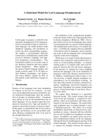
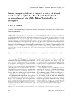
Equation (8) explained 99.5% of the total variance of the
data, and its RMSE was 0.552 m. In selecting the base age, it
was found that 20 years was superior for predicting height at
other ages. The curves for site indices of 11, 16, 21 and 25 m
at a reference age of 20 years overlaid on the profile plots of
the data set are shown in Figure 1.
3.2. Transition function for reduction in tree number
A dynamic equation considering only one parameter to be
site-specific in the base model (Eq. (1)) described the data ad-
equately:
N =

N
−0.3161
0
+ 1.053

t−100
− 1.053
t
0
−100

−1/0.3161
(9)
where N
0
and t
0
represent the predictor number of trees per
hectare and age (years), and N is the predicted number of trees
per hectare at age t.
1
Although they were not developed in the present study, the site qual-
ity system developed by Diéguez-Aranda et al. (2005) and the gener-
alized h-d equation developed by Castedo et al. (2006) are included
in the Results section as part of a summary of all of the components
of the dynamic whole-stand model.
460 F. Castedo-Dorado et al.
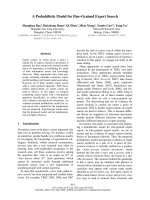
Figure 1. Curves for site indices of 11, 16, 21 and 25 m at a reference
age of 20 years overlaid on the profile plots of the data set.
Figure 2. Trajectories of observed and predicted stem number over
time. Model projections for initial spacing conditions of 400, 1100,
1800 and 2500 stems per hectare at 10 years.
Equation (9) explained approximately 99.3% of the total
variance of the data and the RMSE was 54.8 trees/ha. The tra-
jectories of observed and predicted number of trees over time

for different initial spacing conditions are shown in Figure 2.
3.3. Transition function for stand basal area growth
Of the equations analysed, the models with two site-specific
parameters provided similar results for projecting stand basal
area over time. However, taking into account the adequate
graphs (Fig. 3) and the high predictive ability of the model,
as inferred from the goodness of fit statistics (R
2
= 0.994;
RMSE = 1.29 m
2
ha
−1
), a dynamic model derived from the
Figure 3. Stand basal area growth curves for stand basal areas of
15, 30, 45 and 60 m
2
ha
−1
at 20 years overlaid on the trajectories of
observed values over time.
Korf equation was selected. The model is expressed as fol-
lows:
G = exp
(
X
0
)
exp


−
(
−276.1 + 1391/X
0
)
t
−0.9233

, with
X
0
= 0.5t
−0.9233
0

− 276.1 + t
0.9233
0
ln
(
G
0
)
+

4 × 1391t
0.9233
0
+


276.1 − t
0.9233
0
ln
(
G
0
)

2







(10)
where G
0
and t
0
represent the predictor stand basal area
(m
2
ha
−1
) and age (years), and G is the predicted stand basal
area at age t.
The Korf base equation was also used to develop a stand

basal area initialization function. The previously estimated pa-
rameters of the projection equation were substituted into the
initialization equation, and the unknown site-dependent func-
tion X of the projection function was related to the inverse of
the number of trees per hectare together with a power function
of the site index:
G = exp
(
X
0
)
exp

−
(
−276.1 + 1391/X
0
)
t
−0.9233

, with
X
0
= 4.331SI
0.03594
−
114.3
N
(11)

where G is the predicted stand basal area (m
2
ha
−1
)ataget, N
the number of trees per hectare and SI the site index (m).
3.4. Disaggregation system
3.4.1. Diameter distribution
The equation selected for predicting arithmetic mean diam-
eter and for use in the parameter recovery approach was:
¯
d = d
g
− e
0.1449−19.76
1
t
+0.0001345N+0.03264SI
(12)
A growth model for Pinus radiata D. Don stands in north-western Spain 461
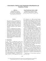
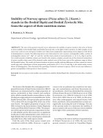
Figure 4. Plots of observed against predicted values of stand volume
for the three time intervals evaluated. The solid line represents the
linear model fitted to the scatter plot of data and the dashed line is the
diagonal. R
2
is the coefficient of determination of the linear model.
where
¯
d is the predicted arithmetic mean diameter (cm), d
g

the quadratic mean diameter (cm), t the stand age (years),
N the number of trees per hectare, and SI the site in-
dex (m). The goodness of fit statistics were R
2
= 0.999 and
RMSE = 0.34 cm.
3.4.2. Height estimation for diameter classes
1
The following generalized h-d relationship was developed
by Castedo et al. [23]:
h =

1.3
0.9339
+

H
0.9339
− 1.3
0.9339

1 − exp
−0.0661d
1 − exp
−0.0661D
0

1/0.9339
(13)
where h is the predicted total height (m) of the subject tree,

d its diameter at breast height (cm), and D
0
and H are dom-
inant diameter and dominant height (the mean diameter and
mean height of the 100 thickest trees per hectare, respectively)
of the stand where the subject tree is included.
This modified expression of the Schnute function showed a
high predictive ability (R
2
= 0.945; RMSE = 1.51 m), and is
very parsimonious (it only depends on two stand variables).
3.4.3. Total and merchantable volume estimation
For total and merchantable volume estimation of the aver-
age tree in each diameter class, the compatible system pro-
posed by Fang et al. [43] was selected. It is constituted by the
following components:
Taper function:
d
i
= c
1

h
(
k−b
1
)
/b
1
(

1 − q
i
)
(
k−β
)
/β
α
I
1
+I
2
1
α
I
2
2
(14)
where







I
1
= 1ifp
1

≤ q
i
≤ p
2
; 0 otherwise
I
2
= 1ifp
2
< q
i
≤ 1; 0 otherwise
p
1
and p
2
are relative heights from ground level where the two
inflection points assumed in the model occur
β = b
1−
(
I
1
+I
2
)
1
b
I
1

2
b
I
2
3
α
1
=
(
1 − p
1
)
(
b
2
−b
1
)
k
b
1
b
2
α
2
=
(
1 − p
2
)

(
b
3
−b
2
)
k
b
2
b
3
r
0
=
(
1 − h
st
/h
)
k/b
1
r
1
=
(
1 − p
1
)
k/b
1

r
2
=
(
1 − p
2
)
k/b
2
c
1
=

a
0
d
a
1
h
a
2
−k/b
1
b
1
(
r
0
− r
1

)
+ b
2
(
r
1
− α
1
r
2
)
+ b
3
α
1
r
2
.
Merchantable volume equation:
v
i
= c
2
1
h
k/b
1

b
1

r
0
+
(
I
1
+ I
2
)(
b
2
− b
1
)
r
1
+ I
2
(
b
3
− b
2
)
α
1
r
2
− β
(

1 − q
i
)
k/β
α
I
1
+I
2
1
α
I
2
2

. (15)
Volume equation:
v = a
0
d
a
1
h
a
2
. (16)
A third-order continuous autoregressive error structure was
necessary to correct the inherent serial autocorrelation of the
experimental stem data. The model provided a very good data
fit, explaining 98.9% of the total variance of d

i
. Moreover, this
model showed few problems associated with multicollinearity.
462 F. Castedo-Dorado et al.
The resulting parameter estimates were:
a
0
:5.293 · 10
−5
; a
1
:1.884; a
2
:0.9777; b
1
:9.193 · 10
−6
;
b
2
:3.282 · 10
−5
; b
3
:2.905 · 10
−5
; p
1
:0.06832; p
2

:0.6566.
The following notation was used: d = diameter at breast height
over bark (cm); d
i
= top diameter at height h
i
over bark (cm);
h = total tree height (m); h
i
= height above the ground to top
diameter d
i
(m); h
st
= stump height (m); v = total tree volume
over bark (m
3
) above stump level; v
i
= merchantable volume
over bark (m
3
), the volume from stump level to a specified top
diameter d
i
; a
0
, a
1
, a

2
, b
1
, b
2
, b
3
, p
1
, p
2
= regression coeffi-
cients to be estimated; k = π/40 000, metric constant to con-
vert from diameter squared in cm
2
to cross-section area in m
2
;
q
i
= h
i
/h.
3.5. Overall evaluation of the model
The growth model described above is comprehensive be-
cause it addresses all forest variables commonly incorporated
in quantitative descriptions of forest growth. The method of
construction adopted is robust because it is based on only three
stand variables; any other variables are derived by auxiliary re-
lationships.

As judged by the observed extrapolation properties, the be-
haviour of the different components is logical for ages close
to the rotation length usually applied to radiata pine stands in
Galicia (25−35 years) (see Figs. 1−3). Moreover, the model
can efficiently project stand development starting from dif-
ferent spacing conditions and considering different thinning
schedules.
To assess if the model satisfies specified accuracy require-
ments, observed dominant height, number of trees per hectare
and stand basal area from the first and second inventory of
the 179 and 46 plots measured two and three times, respec-
tively, served as initial values for the corresponding transition
functions (Eqs. (8), (9), and (10)). These equations were used
to project the stand state at the ages of the second and third
inventory. Equation (12) was then used to estimate the arith-
metic mean diameter, which allowed calculation of the vari-
ance of the diameter distribution. Equations (3) and (4) were
used to recover the Weibull parameters, which allowed esti-
mation of the number of trees in each diameter class. Equa-
tions (13) and (16) were used to estimate the height and the
total volume of the average tree in each diameter class, re-
spectively. Aggregation of total tree volume multiplied by the
number of trees in each diameter class provided total stand
volume.
A plot of observed against predicted values of stand volume
obtained following the above procedure for the three time in-
tervals considered (3, 6 and 9 years) is shown in Figure 4. The
linear model fitted for each scatter plot behaved well in all
three cases (R
2

= 0.984, 0.952 and 0.901, respectively). The
plot also showed that there were no systematic over- or under-
estimates of stand volume for prediction intervals of three and
six years; however, there was a slight tendency towards under-
estimation for a time interval of nine years. Critical errors of
10.9%, 11.9% and 17.3% were obtained for projecting total
stand volume for time intervals of 3, 6 and 9 years, respec-
tively.
4. DISCUSSION
This study presents a whole-stand growth model for ra-
diata pine plantations in north-western Spain, based on the
state-space approach outlined by García [50]. The state of a
stand was adequately described by the following state vari-
ables: dominant height, number of trees per hectare and stand
basal area. The behaviour of the system is described by the rate
of change of these state variables given by their corresponding
transition functions. In addition, other stand variables of inter-
est (quadratic mean diameter, total or merchantable volume,
etc.) can be obtained from the current values of the state vari-
ables. According to this basic structure, the whole-stand model
requires five stand-level inputs for simulation: the age of the
stand at the beginning and the end of the projection interval,
and the initial dominant height, number of trees per hectare
and stand basal area.
All the transition functions used have a theoretical basis,
and have been developed using a recently developed technique
for dynamic equation derivation (GADA: [28]), which ensures
that base-age and path invariance properties provide consis-
tent predictions. Furthermore, the functions were fitted using
a base-age invariant method that accounts for site-specific and

global effects [29].
Dominant height growth transition function consistently
provided accurate values of site indices from heights and ages,
and accurate values of heights from age and site indices, re-
gardless of the levels of site productivity. This is important as
height growth transition function is one of the basic submodels
in whole-stand and other type of growth models (e.g., [53,89]).
The accuracy of the stand survival function over a wide
range of ages and other stand conditions ensures that the pro-
jections of the final output variables of the whole model (e.g.,
stand or merchantable volume) are realistic. This equation is
especially important when light thinnings are carried out [5],
as was the case in most of the studied stands. After heavy thin-
ning operations it seems reasonable to assume that mortality is
negligible.
As regards the stand basal area projection equation, initial
basal area and initial age provided sufficient information about
the future trajectory of the basal area of the stand, regardless
its thinning history. Therefore, the thinning effect is built into
the model, in accordance with the studies of other authors for
several species and regions [8,20, 71]. It must also be consid-
ered that the basal area initialization equation will work well
in unthinned or lightly thinned stands younger than 15 years
(similar to those where the experimental data were collected).
Because the number of trees per hectare varies over time, the
initialization and the projection functions are not compatible.
However, this is not a major problem because the initializa-
tion function would only be used to provide an initial value of
stand basal area when no inventory data are available [4].
A growth model for Pinus radiata D. Don stands in north-western Spain 463

Explanatory variables of the components of the disaggrega-
tion system can be easily obtained at any point in time from
dominant height, number of trees and basal area transition
functions. The only exception is dominant diameter of the gen-
eralized h-d relationship, which is a variable that is difficult to
project [64] and must therefore be estimated from the diameter
distribution.
Total stand volume was selected in the present study as the
critical output variable for the whole-stand growth model, al-
though other stand variables can be assessed on the basis of
this model (e.g., biomass, carbon pools). The allometric equa-
tions for different biomass fractions developed for this species
by Merino et al. [72], which use the diameter at breast height
and the total height as independent variables, can, for exam-
ple, be easily incorporated into the disaggregation system pro-
posed.
The global whole-stand growth model presented was
demonstrated to be robust for medium term projections of
stand volume, even outside the domains of the database used
in its construction. Considering the required accuracy in forest
growth modelling, where a mean prediction error of the ob-
served mean at 95% confidence intervals within ±10%−20%
is generally realistic and reasonable as a limit for the actual
choice of the acceptance and rejection levels [55], we can state
that, on the basis of the critical error statistic obtained, the
model provides satisfactory predictions even for the longest
projection interval (nine years). Nevertheless, for long-term
projections, direct volume estimations for six-year intervals
are recommended. This alternative approach implies the avail-
ability of a new inventory of the stand every six years, but al-

lows reduction, by almost a third, of the critical error of stand
volume estimations.
The relatively simple structure of the growth model makes
it suitable for embedding into landscape-level planning mod-
els and other decision support systems that enable forest man-
agers to generate optimal management strategies. Neverthe-
less, because of the large number of calculations needed to
obtain outputs (especially those involving use of the disag-
gregation system), the model was implemented into a forest
growth simulator called GesMO [22,38] to facilitate its use by
forest managers.
Acknowledgements: This study was financed by the Spanish Min-
istry of Education and Science; project No AGL2004-07976-C02-01.
We thank Dr. Christine Francis for correcting the English grammar of
the text.
REFERENCES
[1] Álvarez Álvarez P., Viveros forestales y uso de planta en re-
población en Galicia, Ph.D. thesis, Universidade de Santiago de
Compostela, 2004.
[2] Álvarez González J.G., Ruiz A., Análisis y modelización de las dis-
tribuciones diamétricas de Pinus pinaster Ait. en Galicia, Investig.
Agrar. Sist. Recur. For. 7 (1998) 123−137.
[3] Álvarez González J.G., Castedo F., Ruiz A.D., López Sánchez C.A.,
Gadow K.v., A two-step mortality model for even-aged stands of
Pinus radiata D. Don in Galicia (north-western Spain), Ann. For.
Sci. 61 (2004) 439−448.
[4] Amateis R.L., Radtke P.J., Burkhart H.E., TAUYIELD: A stand-
level growth and yield model for thinned and unthinned loblolly
pine plantations, Va. Polytech. Inst. State Univ. Sch. For. Wildl.
Resour. Report No. 82, 1995.

[5] Avila O.B., Burkhart H.E., Modeling survival of loblolly pine trees
in thinned and unthinned plantations, Can. J. For. Res. 22 (1992)
1878–1882.
[6] Bailey R.L., Clutter J.L., Base-age invariant polymorphic site
curves, For. Sci. 20 (1974) 155−159.
[7] Bailey R.L., Dell T.R., Quantifying diameter distributions with the
Weibull function, For. Sci. 19 (1973) 97−104.
[8] Barrrio M., Castedo F., Diéguez-Aranda U., Álvarez J.G., Parresol
B.R., Rodríguez R., Development of a basal area growth system for
maritime pine in northwestern Spain using the generalized algebraic
difference approach, Can. J. For. Res. 36 (2006) 1461−1474.
[9] Battaglia M., Sands P.J., Process-based forest productivity models
and their application in forest management, For. Ecol. Manage. 102
(1998) 13−32.
[10] Bertalanffy L.v., Problems of organic growth, Nature 163 (1949)
156−158.
[11] Bertalanffy L.v., Quantitative laws in metabolism and growth, Q.
Rev. Biol. 32 (1957) 217−231.
[12] Borders B.E., Patterson W.D., Projecting stand tables: a compari-
son of the Weibull diameter distribution method, a percentile-based
projection method and a basal area growth projection method, For.
Sci. 36 (1990) 413−424.
[13] Bravo-Oviedo A., Río M. Del., Montero G., Site index curves and
growth model for Mediterranean maritime pine (Pinus pinaster
Ait.) in Spain, For. Ecol. Manage. 201 (2004) 187−197.
[14] Burk T.E., Burkhart H.E., Diameter distributions and yields of
natural stands of loblolly pine, School of Forestry and Wildlife
Resources, VPI and SU, Publication No. FSW-1-84, 1984.
[15] Burk T.E., Newberry J.D., A simple algorithm for moment-based
recovery of Weibull distribution parameters, For. Sci. 30 (1984)

329−332.
[16] Burkhart H.E., Cubic-foot volume of loblolly pine to any mer-
chantable top limit, South. J. Appl. For. 1 (1977) 7−9.
[17] Burkhart H.E., Suggestions for choosing an appropriate level
for modelling forest stands, in: Amaro A., Reed D., Soares P.
(Eds.), Modelling Forest Systems, CAB International, Wallingford,
Oxfordshire, UK, 2003, pp. 3−10.
[18] Cao Q.V., Predicting parameters of a Weibull function for modelling
diameter distributions, For. Sci. 50 (2004) 682−685.
[19] Cao Q.V., Burkhart H.E., A segmented distribution approach for
modeling diameter frequency data, For. Sci. 30 (1984) 129−137.
[20] Cao Q.V., Burkhart H.E., Lemin R.C., Diameter distributions and
yields of thinned loblolly pine plantations, School of Forestry and
Wildlife Resources, VPI and SU, Publication No. FSW-1-82, 1982.
[21] Carmean W.H., Site index curves for upland oaks in the central
states, For. Sci. 18 (1972) 109−120.
[22] Castedo F., Modelo dinámico de crecimiento para las masas de
Pinus radiata D. Don en Galicia. Simulación de alternativas selví-
colas con inclusión del riesgo de incendio, Ph.D. thesis, Universidad
de Santiago de Compostela, 2004.
[23] Castedo F., Diéguez-Aranda U., Barrio M., Sánchez M., Gadow
K.v., A generalized height-diameter model including random com-
ponents for radiata pine plantations in northwestern Spain, For.
Ecol. Manage. 229 (2006) 202−213.
[24] Cieszewski C.J., Three methods of deriving advanced dynamic site
equations demonstrated on inland Douglas-fir site curves, Can. J.
For. Res. 31 (2001) 165−173.
[25] Cieszewski C.J., Comparing fixed- and variable-base-age site equa-
tions having single versus multiple asymptotes, For. Sci. 48 (2002)
7−23.

464 F. Castedo-Dorado et al.
[26] Cieszewski C.J., Developing a well-behaved dynamic site equation
using a modified Hossfeld IV function Y
3
= (ax
m
)/(c + x
m−1
), a
simplified mixed-model and scant subalpine fir data, For. Sci. 49
(2003) 539−554.
[27] Cieszewski C.J., GADA derivation of dynamic site equations with
polymorphism and variable asymptotes from Richards, Weibull,
and other exponential functions, University of Georgia PMRC-TR
2004-5, 2004.
[28] Cieszewski C.J., Bailey R.L., Generalized algebraic difference
approach: Theory based derivation of dynamic site equations
with polymorphism and variable asymptotes, For. Sci. 46 (2000)
116−126.
[29] Cieszewski C.J., Harrison M., Martin S.W., Practical methods for
estimating non-biased parameters in self-referencing growth and
yield models, University of Georgia PMRC-TR 2000-7, 2000.
[30] Clutter J.L., Development of taper functions from variable-top mer-
chantable volume equations, For. Sci. 26 (1980) 117−120.
[31] Clutter J.L., Fortson J.C., Pienaar L.V., Brister H.G., Bailey R.L.,
Timber management: A quantitative approach, John Wiley and Sons
Inc., New York, 1983.
[32] Clutter J.L., Harms W.R., Brister G.H., Rheney J.W., Stand struc-
ture and yields of site-prepared loblolly pine plantations in the
Lower Coastal Plain of the Carolinas, Georgia and north Florida,

USDA Forest Service, Gen. Tech. Rep. SE-27, 1984.
[33] Corral, J.J., Diéguez-Aranda U., Corral S., Castedo F., A mer-
chantable volume system for major pine species in El Salto,
Durango (Mexico), For. Ecol. Manage. 238 (2007) 118−129.
[34] Curtis R.O., Height-diameter and height-diameter-age equations for
second growth Douglas-fir, For. Sci. 13 (1967) 365−375.
[35] Curtis R.O., DeMars D.J., Herman F.R., Which dependent variables
in site index-height-age regressions? For. Sci. 20 (1974) 74−87.
[36] Davis L.S., Johnson K.N., Bettinger P.S., Howard T.E., Forest
management: To sustain ecological, economic, and social values,
McGraw-Hill, New York, 2001.
[37] Demaerschalk J., Converting volume equations to compatible taper
equations, For. Sci. 18 (1972) 241−245.
[38] Diéguez-Aranda U. Modelo dinámico de crecimiento para masas
de Pinus sylvestris L. procedentes de repoblación en Galicia, Ph.D.
thesis, Universidad de Santiago de Compostela, 2004.
[39] Diéguez-Aranda U., Burkhart H.E., Rodríguez R. Modelling dom-
inant height growth of radiata pine (Pinus radiata D. Don) plan-
tations in northwest of Spain, For. Ecol. Manage. 215 (2005)
271−284.
[40] Diéguez-Aranda U., Castedo F., Álvarez J.G., Rojo A., Dynamic
growth model for Scots pine (Pinus sylvestris L.) plantations in
Galicia (north-western Spain), Ecol. Model. 191 (2006) 225−242.
[41] Diéguez-Aranda U., Castedo F., Álvarez J.G., Rojo A., Compatible
taper function for Scots pine (Pinus sylvestris L.) plantations in
north-western Spain, Can. J. For. Res. 36 (2006) 1190−1205.
[42] Falcao A.O., Borges J.G., Designing decision support tools for
Mediterranean forest ecosystems management: a case study in
Portugal, Ann. For. Sci. 62 (2005) 751−760.
[43] Fang Z., Borders B.E., Bailey R.L., Compatible volume-taper mod-

els for loblolly and slash pine based on a system with segmented-
stem form factors, For. Sci. 46 (2000) 1−12.
[44] Frazier J.R., Compatible whole-stand and diameter distribution
models for loblolly pine, Unpublished Ph.D. thesis, VPI and SU,
1981.
[45] Freese F., Testing accuracy, For. Sci. 6 (1960) 139−145.
[46] Gadow K.v., Modelling growth in managed forests – realism and
limits of lumping, Sci. Total Environ. 183 (1996) 167−177.
[47] Gadow K.v., Hui, G.Y., Modelling forest development, Kluwer
Academic Publishers, Dordrecht, 1999.
[48] García O., Growth modelling – a (re)view, N. Z. For. 33 (1988)
14−17.
[49] García O., Growth of thinned and pruned stands, in: James R.Ñ.,
Tarlton G.L. (Eds.), Proceedings of a IUFRO Symposium on
New Approaches to Spacing and Thinning in Plantation Forestry.
Rotorua, New Zealand, Ministry of Forestry, FRI Bulletin No. 151,
1990, pp. 84−97.
[50] García O., The state-space approach in growth modelling, Can. J.
For. Res. 24 (1994) 1894−1903.
[51] García O., Dimensionality reduction in growth models: an exam-
ple, Forest biometry, Modelling and Information Sciences 1 (2003)
1−15.
[52] García O., Ruiz F., A growth model for eucalypt in Galicia, Spain,
For. Ecol. Manage. 173 (2003) 49−62.
[53] Hein S., Dhote J.F., Effect of species composition, stand density
and site index on the basal area increment of oak trees (Quercus
sp.) in mixed stands with beech (Fagus sylvatica L.) in Northern
France, Ann. For. Sci. 63 (2006) 457−467.
[54] Hossfeld J.W., Mathematik für Forstmänner, Ökonomen und
Cameralisten (Gotha, 4. Bd., S. 310), 1882.

[55] Huang S., Yang Y., Wang Y., A critical look at procedures for val-
idating growth and yield models, in: Amaro A., Reed D., Soares P.
(Eds.), Modelling Forest Systems, CAB International, Wallingford,
Oxfordshire, UK, 2003, pp. 271−293.
[56] Hyink D.M., Diameter distribution approaches to growth and yield
modelling, in: Brown K.M., Clarke F.R. (Eds.), Forecasting forest
stand dynamics, School of Forestry, Lakehead University, 1980, pp.
138−163.
[57] Hyink D.M., Moser J.W., A generalized framework for projecting
forest yield and stand structure using diameter distributions, For.
Sci. 29 (1983) 85−95.
[58] Kangas A., Maltamo M., Calibrating predicted diameter distribution
with additional information, For. Sci. 46 (2000) 390−396.
[59] Knoebel B.R., Burkhart H.E., Beck D.E., A growth and yield model
for thinned stands of yellow-poplar, For. Sci. Monogr. 27, 1986.
[60] Kotze H., A strategy for growth and yield research in pine and eu-
calipt plantations in Komatiland Forests in South Africa, in: Amaro
A., Reed D., Soares P. (Eds.), Modelling Forest Systems, CAB
International, Wallingford, Oxfordshire, UK, 2003, pp. 75−84.
[61] Kozak A., Effects of multicollinearity and autocorrelation on the
variable-exponent taper functions, Can. J. For. Res. 27 (1997)
619−629.
[62] Kozak A., My last words on taper functions, For. Chron. 80 (2004)
507−515.
[63] Kozak A., Kozak R., Does cross validation provide additional infor-
mation in the evaluation of regression models? Can. J. For. Res. 33
(2003) 976−987.
[64] Lappi J., A longitudinal analysis of height/diameter curves, For. Sci.
43 (1997) 555−570.
[65] Lei Y., Parresol B.R., Remarks on height-diameter modelling,

USDA Forest Service Research Note SRS-10, 2001.
[66] López C.A., Gorgoso J.J., Castedo F., Rojo A., Rodríguez R.,
Álvarez J.G., Sánchez F., A height-diameter model for Pinus ra-
diata D. Don in Galicia (northwest Spain), Ann. For. Sci. 60 (2003)
237−245.
[67] Lundqvist B., On the height growth in cultivated stands of pine
and spruce in northern Sweden, Medd. Fran Statens Skogforsk 47
(1957) 1−64.
[68] Mabvurira D., Maltamo M., Kangas A., Predicting and calibrating
diameter distributions of Eucalyptus grandis (Hill) Maiden planta-
tions in Zimbabwe, New. For. 23 (2002) 207−223.
[69] Maltamo M., Puumalainen J., Päivinen R., Comparison of Beta and
Weibull functions for modelling basal area diameter distributions in
stands of Pinus sylvestris and Picea abies, Scand. J. For. Res. 10
(1995) 284−295.
A growth model for Pinus radiata D. Don stands in north-western Spain 465
[70] MAPA, Anuario de Estadística Agroalimentaria 2003, Ministerio
de Agricultura, Pesca y Alimentación, Subdirección General de
Estadísticas Agroalimentarias, Secretaria General Técnica, 2004.
[71] Matney T.G., Sullivan A.D., Compatible stand and stock tables for
thinned and unthinned loblolly pine stands, For. Sci. 28 (1982)
161−171.
[72] Merino A., Balboa M.A., Rodríguez R., Álvarez J.G., Nutrient
exports under different harvesting regimes in fast-growing forest
plantations in southern Europe, For. Ecol. Manage. 207 (2005)
325−339.
[73] Milsum J.H., Biological Control Systems Analysis, McGraw-Hill,
New York, 1966.
[74] Monserud R.A., Height growth and site index curves for inland
Douglas-fir based on stem analysis data and forest habitat type, For.

Sci. 30 (1984) 943−965.
[75] Newberry J.D., A note on Carmean’s estimate of height from stem
analysis data, For. Sci. 37 (1991) 368−369.
[76] Newby M., The properties of moment estimators for the
Weibull distribution based on the sample coefficient of variation,
Technometrics 22 (1980) 187−194.
[77] Northway S.M., Fitting site index equations and other self-
referencing functions, For. Sci. 31 (1985) 233−235.
[78] Parresol B.R., Recovering parameters of Johnson’s SB distribution,
USDA Forest Service, Res. Pap. SRS-31, 2003.
[79] Peet R.K., Christensen N.L., Competition and tree death,
Bioscience 37 (1987) 586−595.
[80] Pienaar L.V., Turnbull K.J., The Chapman-Richards generalization
of von Bertalanffy’s growth model for basal area growth and yield
in even-aged stands, For. Sci. 19 (1973) 2−22.
[81] Pinjuv G., Mason E.G., Watt M., Quantitative validation and com-
parison of a range of forest growth model types, For. Ecol. Manage.
236 (2006) 37–46.
[82] Reynolds M.R. Jr., Estimating the error in model predictions, For.
Sci. 30 (1984) 454−469.
[83] Reynolds M.R.Jr., Burk T.E., Huang W.C., Goodness-of-fit tests and
model selection procedures for diameter distributions models, For.
Sci. 34 (1988) 373−399.
[84] Richards F.J., A flexible growth function for empirical use, J. Exp.
Bot. 10 (1959) 290−300.
[85] Río M. del, Régimen de claras y modelo de producción para Pinus
sylvestris L. en los Sistemas Central e Ibérico, Tesis Doctorales
INIA No. 2, Serie Forestal, 1999.
[86] Robinson A.P., Froese R.E., Model validation using equivalence
tests, Ecol. Model. 176 (2004) 349−358.

[87] Rykiel E.J., Testing ecological models: the meaning of validation,
Ecol. Model. 90 (1996) 229−244.
[88] Sánchez F., Rodríguez R., Rojo A., Álvarez J.G., López C., Gorgoso
J., Castedo F., Crecimiento y tablas de producción de Pinus radi-
ata D. Don en Galicia, Investig. Agrar. Sist. Recur. For. 12 (2003)
65−83.
[89] Sanchez-Gonzalez M., Tomé M., Montero G., Modelling height and
diameter growth of dominant cork oak in Spain, Ann. For. Sci. 62
(2006) 633−643.
[90] Sargent R.G., Validation and verification of simulation models, in:
Proceedings of the 1999 Winter Simulation Conference, Farrington
H.B. et al. (Eds.), Institute of Electrical and Electronic Engineers,
New York, 1999, pp. 39−48.
[91] SAS Institute Inc., SAS/ETS

9.1 User’s Guide, Cary, NC: SAS
Institute Inc., 2004.
[92] Schnute J., A versatile growth model with statistically stable param-
eters, Can. J. Fish. Aquatic. Sci. 38 (1981) 1128−1140.
[93] Sharma M., Zhang S.Y., Height-diameter models using stand char-
acteristics for Pinus banksiana and Picea mariana, Scand. J. For.
Res. 19 (2004) 442−451.
[94] Tickle P.K., Coops N.C., Hafner S.D., The Bago Science Team,
Assessing forest productivity at local scales across a native euca-
lypt forest using a process-based model, 3PG-SPATIAL, For. Ecol.
Manage. 152 (2001) 275−291.
[95] Torres-Rojo J.M., Magaña-Torres O.S., Acosta-Mireles M.,
Metodología para mejorar la predicción de parámetros de distribu-
ciones diamétricas, Agrociencia 34 (2000) 627−637.
[96] Trincado G.V., Quezada P.R., Gadow K.v., A Comparison of

two stand table projection methods for young Eucalyptus nitens
(Maiden) plantations in Chile, For. Ecol. Manage. 180 (2003)
443−451.
[97] Uribe A., Modelación del crecimiento de Pinus patula Schletch et
Cham en la región Andina suroccidental colombiana, in: Ortega
A., Gezan S. (Eds.), Proceedings of the IUFRO Conference on
Modelling Growth of Fast-Grown Tree Species, Valdivia (Chile),
1997, pp. 36−51.
[98] Vanclay J.K., Modelling forest growth and yield. Applications to
mixed tropical forests, CAB International, Wallingford, UK, 1994.
[99] Vanclay J.K., Growth models for tropical forests: a synthesis of
models and methods, For. Sci. 41 (1995) 7−42.
[100] Vanclay J.K., Skovsgaard J.P., Evaluating forest growth models,
Ecol. Model. 98 (1997) 1−12.
[101] Woollons R.C., Even-aged stand mortality estimation through
a two-step regression process, For. Ecol. Manage. 105 (1998)
189−195.
[102] Xunta de Galicia, O monte galego en cifras. Dirección Xeral
de Montes e Medio Ambiente Natural, Consellería de Medio
Ambiente, Santiago de Compostela, 2001.
[103] Yang Y., Monserud R.A., Huang S., An evaluation of diagnostic
test and their roles in validating forest biometric models, Can. J.
For. Res. 34 (2004) 619−629.
[104] Zarnoch S.J., Feduccia D.P., Baldwin V.C., Dell T.R., Growth and
yield predictions for thinned and unthinned slash pine plantations
on cutover sites in the West Gulf region, USDA Forest Service, Res.
Pap. SO-264, 1991.
[105] Zimmerman D.L., Núñez-Antón V., Parametric modelling of
growth curve data: An overview (with discussion), Test 10 (2001)
1−73.