- Trang chủ >>
- Khoa Học Tự Nhiên >>
- Vật lý
CHAPTER 11: THE UNIFORM PLANE WAVEIn ppt
Bạn đang xem bản rút gọn của tài liệu. Xem và tải ngay bản đầy đủ của tài liệu tại đây (937.35 KB, 39 trang )
CHAPTER
11
THE
UNIFORM
PLANE
WAVE
In this chapter we shall apply Maxwell's equations to introduce the fundamental
theory of wave motion. The uniform plane represents one of the simplest appli-
cations of Maxwell's equations, and yet it is of profound importance, since it is a
basic entity by which energy is propagated. We shall explore the physical pro-
cesses that determine the speed of propagation and the extent to which attenua-
tion may occur. We shall derive and make use of the Poynting theorem to find
the power carried by a wave. Finally, we shall learn how to describe wave
polarization. This chapter is the foundation for our explorations in later chapters
which will include wave reflection, basic transmission line and waveguiding con-
cepts, and wave generation through antennas.
11.1 WAVE PROPAGATION IN FREE SPACE
As we indicated in our discussion of boundary conditions in the previous chap-
ter, the solution of Maxwell's equations without the application of any boundary
conditions at all represents a very special type of problem. Although we restrict
our attention to a solution in rectangular coordinates, it may seem even then that
we are solving several different problems as we consider various special cases in
this chapter. Solutions are obtained first for free-space conditions, then for
perfect dielectrics, next for lossy dielectrics, and finally for the good conductor.
We do this to take advantage of the approximations that are applicable to each
348
| | | |
▲
▲
e-Text Main Menu
Textbook Table of Contents
special case and to emphasize the special characteristics of wave propagation in
these media, but it is not necessary to use a separate treatment; it is possible (and
not very difficult) to solve the general problem once and for all.
To consider wave motion in free space first, Maxwell's equations may be
written in terms of E and H only as
rÂH
0
@E
@t
1
rÂE À
0
@H
@t
2
rÁE 0 3
rÁH 0 4
Now let us see whether wave motion can be inferred from these four equa-
tions without actually solving them. The first equation states that if E is changing
with time at some point, then H has curl at that point and thus can be considered
as forming a small closed loop linking the changing E field. Also, if E is changing
with time, then H will in general also change with time, although not necessarily
in the same way. Next, we see from the second equation that this changing H
produces an electric field which forms small closed loops about the H lines. We
now have once more a changing electric field, our original hypothesis, but this
field is present a small distance away from the point of the original disturbance.
We might guess (correctly) that the velocity with which the effect moves away
from the original point is the velocity of light, but this must be checked by a more
quantitative examination of Maxwell's equations.
Let us first write Maxwell's four equations above for the special case of
sinusoidal (more strictly, cosinusoidal) variation with time. This is accomplished
by complex notation and phasors. The procedure is identical to the one we used
in studying the sinusoidal steady state in electric circuit theory.
Given the vector field
E E
x
a
x
we assume that the component E
x
is given as
E
x
Ex; y; zcos!t 5
where Ex; y; z is a real function of x; y; z and perhaps !, but not of time, and
is a phase angle which may also be a function of x; y; z and !. Making use of
Euler's identity,
e
j!t
cos !t j sin !t
we let
E
x
ReEx; y; ze
j!t
ReEx; y; ze
j
e
j!t
6
THE UNIFORM PLANE WAVE 349
| | | |
▲
▲
e-Text Main Menu
Textbook Table of Contents
where Re signifies that the real part of the following quantity is to be taken. If we
then simplify the nomenclature by dropping Re and suppressing e
j!t
, the field
quantity E
x
becomes a phasor, or a complex quantity, which we identify by use
of an s subscript, E
xs
. Thus
E
xs
Ex; y; ze
j
7
and
E
s
E
xs
a
x
The s can be thought of as indicating a frequency domain quantity expressed as a
function of the complex frequency s, even though we shall consider only those
cases in which s is a pure imaginary, s j!.
h
Example 11.1
Let us express E
y
100 cos10
8
t À 0:5z 308 V/m as a phasor.
Solution. We first go to exponential notation,
E
y
Re100e
j10
8
tÀ0:5z308
and then drop Re and suppress e
j10
8
t
, obtaining the phasor
E
ys
100e
Àj0:5zj308
Note that E
y
is real, but E
ys
is in general complex. Note also that a mixed
nomenclature is commonly used for the angle. That is, 0:5z is in radians, while
308 is in degrees.
Given a scalar component or a vector expressed as a phasor, we may easily
recover the time-domain expression.
h
Example 11.2
Given the field intensity vector, E
s
100308a
x
20À508a
y
402108a
z
V/m, iden-
tified as a phasor by its subscript s, we desire the vector as a real function of time.
Solution. Our starting point is the phasor,
E
s
100308a
x
20À508a
y
402108a
z
V=m
Let us assume that the frequency is specified as 1 MHz. We first select exponential
notation for mathematical clarity,
E
s
100e
j308
a
x
20e
Àj508
a
y
40e
j2108
a
z
V=m
reinsert the e
j!t
factor,
E
s
t100e
j308
a
x
20e
Àj508
a
y
40e
j2108
a
z
e
j210
6
t
100e
j210
6
t308
a
x
20e
j210
6
tÀ508
a
y
40e
j210
6
t2108
a
z
350 ENGINEERING ELECTROMAGNETICS
| | | |
▲
▲
e-Text Main Menu
Textbook Table of Contents
and take the real part, obtaining the real vector,
Et100 cos210
6
t 308a
x
20 cos210
6
t À 508a
y
40 cos210
6
t 2108a
z
None of the amplitudes or phase angles in this example are expressed as a
function of x, y,orz, but, if any are, the same procedure is effective. Thus, if
H
s
20e
À0:1j20z
a
x
A/m, then
HtRe20e
À0:1z
e
Àj20z
e
j!t
a
x
20e
À0:1z
cos!t À20za
x
A=m
Now, since
@E
x
@t
@
@t
Ex; y; zcos!t À!Ex; y; zsin!t
Rej!E
xs
e
j!t
it is evident that taking the partial derivative of any field quantity with respect to
time is equivalent to multiplying the corresponding phasor by j!. As an example,
if
@E
x
@t
À
1
0
@H
y
@z
the corresponding phasor expression is
j!E
xs
À
1
0
@H
ys
@z
where E
xs
and H
ys
are complex quantities. We next apply this notation to
Maxwell's equations. Thus, given the equation,
rÂH
0
@E
@t
the corresponding relationship in terms of phasor-vectors is
rÂH
s
j!
0
E
s
8
Equation (8) and the three equations
rÂE
s
Àj!
0
H
s
9
rÁE
s
0 10
rÁH
s
0 11
are Maxwell's four equations in phasor notation for sinusoidal time variation in
free space. It should be noted that (10) and (11) are no longer independent
relationships, for they can be obtained by taking the divergence of (8) and (9),
respectively.
THE UNIFORM PLANE WAVE 351
| | | |
▲
▲
e-Text Main Menu
Textbook Table of Contents
Our next step is to obtain the sinusoidal steady-state form of the wave
equation, a step we could omit because the simple problem we are going to
solve yields easily to simultaneous solution of the four equations above. The
wave equation is an important equation, however, and it is a convenient starting
point for many other investigations.
The method by which the wave equation is obtained could be accomplished
in one line (using four equals signs on a wider sheet of paper):
rÂrÂE
s
rr Á E
s
Àr
2
E
s
Àj!
0
rÂH
s
!
2
0
0
E
s
Àr
2
E
s
since rÁE
s
0. Thus
r
2
E
s
Àk
2
0
E
s
12
where k
0
, the free space wavenumber, is defined as
k
0
!
0
0
p
13
Eq. (12) is known as the vector Helmholtz equation.
1
It is fairly formidable when
expanded, even in rectangular coordinates, because three scalar phasor equations
result, and each has four terms. The x component of (12) becomes, still using the
del-operator notation,
r
2
E
xs
Àk
2
0
E
xs
14
and the expansion of the operator leads to the second-order partial differential
equation
@
2
E
xs
@x
2
@
2
E
xs
@y
2
@
2
E
xs
@z
2
Àk
2
0
E
xs
15
Let us attempt a solution of (15) by assuming that a simple solution is possible in
which E
xs
does not vary with x or y, so that the two corresponding derivatives
are zero, leading to the ordinary differential equation
d
2
E
xs
dz
2
Àk
2
0
E
xs
16
By inspection, we may write down one solution of (16):
E
xs
E
x0
e
Àjk
0
z
17
352
ENGINEERING ELECTROMAGNETICS
1
Hermann Ludwig Ferdinand von Helmholtz (1821±1894) was a professor at Berlin working in the fields
of physiology, electrodynamics, and optics. Hertz was one of his students.
| | | |
▲
▲
e-Text Main Menu
Textbook Table of Contents
Next, we reinsert the e
j!t
factor and take the real part,
E
x
z; tE
x0
cos!t Àk
0
z18
where the amplitude factor, E
x0
, is the value of E
x
at z 0, t 0. Problem 1 at
the end of the chapter indicates that
E
H
x
z; tE
H
x0
cos!t k
0
z19
may also be obtained from an alternate solution of the vector Helmholtz equa-
tion.
We refer to the solutions expressed in (18) and (19) as the real instantaneous
forms of the electric field. They are the mathematical representations of what one
would experimentally measure. The terms !t and k
0
z, appearing in (18) and (19),
have units of angle, and are usually expressed in radians. We know that ! is the
radian time frequency, measuring phase shift per unit time, and which has units of
rad/sec. In a similar way, we see that k
0
will be interpreted as a spatial frequency,
which in the present case measures the phase shift per unit distance along the z
direction. Its units are rad/m. In addition to its original name (free space wave-
number), k
0
is also the phase constant for a uniform plane wave in free space.
We see that the fields of (18) and (19) are x components, which we might
describe as directed upward at the surface of a plane earth. The radical
0
0
p
,
contained in k
0
, has the approximate value 1=3 Â10
8
s/m, which is the reci-
procal of c, the velocity of light in free space,
c
1
0
0
p
2:998 Â10
8
:
3 Â10
8
m=s
We can thus write k
0
!=c, and Eq. (18), for example, can be rewritten as
E
x
z; tE
x0
cos!t Àz=c 20
The propagation wave nature of the fields as expressed in (18), (19), and (20) can
now be seen. First, suppose we were to fix the time at t 0. Eq. (20) then becomes
E
x
z; 0E
x0
cos
!z
c
E
x0
cosk
0
z21
which we identify as a simple periodic function that repeats every incremental
distance , known as the wavelength. The requirement is that k
0
2, and so
2
k
0
c
f
3 Â10
8
f
(free space) 22
Now suppose we consider some point (such as a wave crest) on the cosine function
of Eq. (21). For a crest to occur, the argument of the cosine must be an integer
multiple of 2. Considering the mth crest of the wave, the condition becomes
THE UNIFORM PLANE WAVE 353
| | | |
▲
▲
e-Text Main Menu
Textbook Table of Contents
k
0
z 2m
So let us now consider the point on the cosine that we have chosen, and see what
happens as time is allowed to increase. Eq. (18) now applies, where our require-
ment is that the entire cosine argument be the same multiple of 2 for all time, in
order to keep track of the chosen point. From (18) and (20) our condition now
becomes
!t Àk
0
z !t Àz=c2m 23
We see that as time increases (as it must), the position z must also increase in
order to satisfy (23). Thus the wave crest (and the entire wave) moves in the
positive z direction. The speed of travel, or wave phase velocity, is given by c
(in free space), as can be deduced from (23). Using similar reasoning, Eq. (19),
having cosine argument !t k
0
z, describes a wave that moves in the negative z
direction, since as time increases, z must now decrease to keep the argument
constant. Waves expressed in the forms exemplified by Eqs. (18) and (19) are
called traveling waves. For simplicity, we will restrict our attention in this chapter
to only the positive z traveling wave.
Let us now return to Maxwell's equations, (8) to (11), and determine the
form of the H field. Given E
s
, H
s
is most easily obtained from (9),
rÂE
s
Àj!
0
H
s
9
which is greatly simplified for a single E
xs
component varying only with z,
dE
xs
dz
Àj!
0
H
ys
Using (17) for E
xs
, we have
H
ys
À
1
j!
0
Àjk
0
E
x0
e
Àjk
0
z
E
x0
0
0
e
Àjk
0
z
In real instantaneous form, this becomes
H
y
z; tE
x0
0
0
cos!t Àk
0
z24
where E
x0
is assumed real.
We therefore find the x-directed E field that propagates in the positive z
direction is accompanied by a y-directed H field. Moreover, the ratio of the
electric and magnetic field intensities, given by the ratio of (18) to (24),
E
x
H
y
0
0
25
is constant. Using the language of circuit theory, we would say that E
x
and H
y
are ``in phase,'' but this in-phase relationship refers to space as well as to time.
We are accustomed to taking this for granted in a circuit problem in which a
354
ENGINEERING ELECTROMAGNETICS
| | | |
▲
▲
e-Text Main Menu
Textbook Table of Contents
current I
m
cos !t is assumed to have its maximum amplitude I
m
throughout an
entire series circuit at t 0. Both (18) and (24) clearly show, however, that the
maximum value of either E
x
or H
y
occurs when !t Àz=c is an integral multiple
of 2 rad; neither field is a maximum everywhere at the same instant. It is
remarkable, then, that the ratio of these two components, both changing in
space and time, should be everywhere a constant.
The square root of the ratio of the permeability to the permittivity is called
the intrinsic impedance (eta),
26
where has the dimension of ohms. The intrinsic impedance of free space is
0
0
0
377
:
120
This wave is called a uniform plane wave because its value is uniform through-
out any plane, z constant. It represents an energy flow in the positive z
direction. Both the electric and magnetic fields are perpendicular to the direc-
tion of propagation, or both lie in a plane that is transverse to the direction of
propagation; the uniform plane wave is a transverse electromagnetic wave,ora
TEM wave.
Some feeling for the way in which the fields vary in space may be
obtained from Figs 11.1a and 11.1b. The electric field intensity in Fig. 11.1a
is shown at t 0, and the instantaneous value of the field is depicted along
three lines, the z axis and arbitrary lines parallel to the z axis in the x 0 and
y 0 planes. Since the field is uniform in planes perpendicular to the z axis,
the variation along all three of the lines is the same. One complete cycle of the
variation occurs in a wavelength, . The values of H
y
at the same time and
positions are shown in Fig. 11.1b.
A uniform plane wave cannot exist physically, for it extends to infinity in
two dimensions at least and represents an infinite amount of energy. The distant
field of a transmitting antenna, however, is essentially a uniform plane wave in
some limited region; for example, a radar signal impinging on a distant target is
closely a uniform plane wave.
Although we have considered only a wave varying sinusoidally in time
and space, a suitable combination of solutions to the wave equation may be
made to achieve a wave of any desired form. The summation of an infinite
number of harmonics through the use of a Fourier series can produce a per-
iodic wave of square or triangular shape in both space and time. Nonperiodic
waves may be obtained from our basic solution by Fourier integral methods.
These topics are among those considered in the more advanced books on
electromagnetic theory.
THE UNIFORM PLANE WAVE 355
| | | |
▲
▲
e-Text Main Menu
Textbook Table of Contents
\ D11.1. The electric field amplitude of a uniform plane wave propagating in the a
z
direction is 250 V/m. If E E
x
a
x
and ! 1:00 Mrad/s, find: (a) the frequency; (b)
the wavelength; (c) the period; (d) the amplitude of H.
Ans. 159 kHz; 1.88 km; 6.28 ms; 0.663 A/m
\ D11.2 Let H
s
2À408a
x
À 3208a
y
e
Àj0:07z
A/m for a uniform plane wave traveling
in free space. Find: (a) !; (b) H
x
at P1; 2; 3 at t 31 ns; (c) jHj at t 0 at the origin.
Ans. 21.0 Mrad/s; 1.93 A/m; 3.22 A/m
11.2 WAVE PROPAGATION IN DIELECTRICS
Let us now extend our analytical treatment of the uniform plane wave to pro-
pagation in a dielectric of permittivity and permeability . The medium is
isotropic and homogeneous, and the wave equation is now
r
2
E
s
Àk
2
E
s
27
where the wavenumber is now a function of the material properties:
k !
p
k
0
R
R
p
28
356
ENGINEERING ELECTROMAGNETICS
FIGURE 11.1
(a) Arrows represent the instantaneous values of E
x0
cos!t Àz=c at t 0 along the z axis, along an
arbitrary line in the x 0 plane parallel to the z axis, and along an arbitrary line in the y 0 plane parallel
to the z axis. (b) Corresponding values of H
y
are indicated. Note that E
x
and H
y
are in phase at any point
at any time.
| | | |
▲
▲
e-Text Main Menu
Textbook Table of Contents
For E
xs
we have
d
2
E
xs
dz
2
Àk
2
E
xs
29
An important feature of wave propagation in a dielectric is that k can be
complex-valued, and as such is referred to as the complex propagation constant.
A general solution of (29) in fact allows the possibility of a complex k, and it is
customary to write it in terms of its real and imaginary parts in the following
way:
jk j 30
A solution of (29) will be:
E
xs
E
x0
e
Àjkz
E
x0
e
Àz
e
Àjz
31
Multiplying (31) by e
j!t
and taking the real part yields a form of the field that
can be more easily visualized:
E
x
E
x0
e
Àz
cos!t Àz32
We recognize the above as a uniform plane wave that propagates in the forward z
direction with phase constant , but which (for positive ) loses amplitude with
increasing z according to the factor e
Àz
. Thus the general effect of a complex-
valued k is to yield a traveling wave that changes its amplitude with distance.If is
positive, it is called the attenuation coefficient.If is negative, the wave grows in
amplitude with distance, and is called the gain coefficient. The latter effect
would occur, for example, in laser amplifiers. In the present and future discus-
sions in this book, we will consider only passive media, in which one or more loss
mechanisms are present, thus producing a positive .
The attenuation coefficient is measured in nepers per meter (Np/m) in order
that the exponent of e be measured in the dimensionless units of nepers.
2
Thus, if
0:01 Np/m, the crest amplitude of the wave at z 50 m will be
e
À0:5
=e
À0
0:607 of its value at z 0. In traveling a distance 1= in the z
direction, the amplitude of the wave is reduced by the familiar factor of e
À1
,
or 0.368.
THE UNIFORM PLANE WAVE 357
2
The term neper was selected (by some poor speller) to honor John Napier, a Scottish mathematician who
first proposed the use of logarithms.
| | | |
▲
▲
e-Text Main Menu
Textbook Table of Contents
The ways in which physical processes in a material can affect the wave
electric field are described through a complex permittivity of the form
H
À j
HH
33
Two important mechanisms that give rise to a complex permittivity (and thus
result in wave losses) are bound electron or ion oscillations and dipole relaxation,
both of which are discussed in Appendix D. An additional mechanism is the
conduction of free electrons or holes, which we will explore at length in this
chapter.
Losses arising from the response of the medium to the magnetic field can
occur as well, and are modeled through a complex permeability,
H
À j
HH
.
Examples of such media include ferrimagnetic materials, or ferrites. The mag-
netic response is usually very weak compared to the dielectric response in most
materials of interest for wave propagation; in such materials %
0
.
Consequently, our discussion of loss mechanisms will be confined to those
described through the complex permittivity.
We can substitute (33) into (28), which results in
k !
H
À j
HH
!
H
1 Àj
HH
H
34
Note the presence of the second radical factor in (34), which becomes unity (and
real) as
HH
vanishes. With non-zero
HH
, k is complex, and so losses occur which
are quantified through the attenuation coefficient, , in (30). The phase constant,
(and consequently the wavelength and phase velocity), will also be affected by
HH
. and are found by taking the real and imaginary parts of jk from (34). We
obtain:
Refjkg!
H
2
1
HH
H
2
À 1
1=2
35
Imfjkg!
H
2
1
HH
H
2
1
1=2
36
We see that a non-zero (and hence loss) results if the imaginary part of the
permittivity,
HH
, is present. We also observe in (35) and (36) the presence of the
ratio
HH
=
H
, which is called the loss tangent. The meaning of the term will be
demonstrated when we investigate the specific case of conductive media. The
practical importance of the ratio lies in its magnitude compared to unity, which
enables simplifications to be made in (35) and (36).
358
ENGINEERING ELECTROMAGNETICS
| | | |
▲
▲
e-Text Main Menu
Textbook Table of Contents
Whether or not losses occur, we see from (32) that the wave phase velocity
is given by
v
p
!
37
The wavelength is the distance required to effect a phase change of 2 radians
2
which leads to the fundamental definition of wavelength,
2
38
Since we have a uniform plane wave, the magnetic field is found through
H
ys
E
x0
e
Àz
e
Àjz
where the intrinsic impedance is now a complex quantity,
H
À j
HH
H
1
1 Àj
HH
=
H
39
The electric and magnetic fields are no longer in phase.
A special case is that of a lossless medium, or perfect dielectric, in which
HH
0, and so
H
. From (35), this leads to 0, and from (36),
!
H
!
p
(lossless medium) 40
With 0, the real field assumes the form:
E
x
E
x0
cos!t Àz41
We may interpret this as a wave traveling in the z direction at a phase velocity
v
p
, where
v
p
!
1
p
c
R
R
p
THE UNIFORM PLANE WAVE 359
| | | |
▲
▲
e-Text Main Menu
Textbook Table of Contents
The wavelength is
2
2
!
p
1
f
p
c
f
R
R
p
0
R
R
p
(lossless medium) 42
where
0
is the free space wavelength. Note that
R
R
> 1, and therefore the
wavelength is shorter and the velocity is lower in all real media than they are in
free space.
Associated with E
x
is the magnetic field intensity
H
y
E
x0
cos!t Àz
where the intrinsic impedance is
43
The two fields are once again perpendicular to each other, perpendicular to
the direction of propagation, and in phase with each other everywhere. Note that
when E is crossed into H, the resultant vector is in the direction of propagation.
We shall see the reason for this when we discuss the Poynting vector.
h
Example 11.3
Let us apply these results to a 1 MHz plane wave propagating in fresh water. At this
frequency, losses in water are known to be small, so for simplicity, we will neglect
HH
.In
water,
R
1 and at 1 MHz,
H
R
R
81.
Solution. We begin by calculating the phase constant. Using (36) with
HH
0, we have
!
H
!
0
0
p
H
R
!
H
R
c
2 Â 10
6
81
p
3:0 Â 10
8
0:19 rad=m
Using this result, we can determine the wavelength and phase velocity:
2
2
:19
33 m
v
p
!
2 Â 10
6
:19
3:3 Â 10
7
m=s
The wavelength in air would have been 300 m. Continuing our calculations, we find the
intrinsic impedance, using (39) with
HH
0:
H
0
H
R
377
9
42
360 ENGINEERING ELECTROMAGNETICS
| | | |
▲
▲
e-Text Main Menu
Textbook Table of Contents
If we let the electric field intensity have a maximum amplitude of 0.1 V/m, then
E
x
0:1 cos210
6
t À :19z V=m
H
y
E
x
2:4 Â 10
À3
cos210
6
t À :19z A=m
\ D11.3. A 9.375-GHz uniform plane wave is propagating in polyethylene (see Appendix
C). If the amplitude of the electric field intensity is 500 V/m and the material is assumed
to be lossless, find: (a) the phase constant; (b) the wavelength in the polyethylene; (c) the
velocity of propagation; (d) the intrinsic impedance; (e) the amplitude of the magnetic
field intensity.
Ans. 295 rad/m; 2.13 cm; 1:99 Â 10
8
m/s; 251 ; 1.99 A/m
h
Example 11.4
We again consider plane wave propagation in water, but at the much higher microwave
frequency of 2.5 GHz. At frequencies in this range and higher, dipole relaxation and
resonance phenomena
3
in the water molecules become important. Real and imaginary
parts of the permittivity are present, and both vary with frequency. At frequencies below
that of visible light, the two mechanisms together produce an
HH
that increases with
increasing frequency, reaching a local maximum in the vicinity of 10
10
Hz.
H
decreases
with increasing frequency. Ref. 3 provides specific details. At 2.5 GHz, dipole relaxation
effects dominate. The permittivity values are
H
R
78 and
HH
R
7. From(35), we have
2 Â 2:5 Â 10
9
78
p
3:0 Â 10
8
2
p
1
7
78
2
À 1
1=2
21 Np=m
The first calculation demonstrates the operating principle of the microwave oven. Almost
all foods contain water, and so can be cooked when incident microwave radiation is
absorbed and converted into heat. Note that the field will attenuate to a value of e
À1
times its initial value at a distance of 1= 4:8 cm. This distance is called the penetra-
tion depth of the material, and of course is frequency-dependent. The 4.8 cm depth is
reasonable for cooking food, since it would lead to a temperature rise that is fairly
uniform throughout the depth of the material. At much higher frequencies, where
HH
is
larger, the penetration depth decreases, and too much power is absorbed at the surface;
at lower frequencies, the penetration depth increases, and not enough overall absorption
occurs. Commercial microwave ovens operate at frequencies in the vicinity of 2.5 GHz.
Using (36), in a calculation very similar to that for , we find 464 rad/m. The
wavelength is 2= 1:4 cm, whereas in free space this would have been
0
c=f 12 cm.
THE UNIFORM PLANE WAVE 361
3
These mechanisms and how they produce a complex permittivity are described in Appendix D.
Additionally, the reader is referred to pp. 73±84 in Ref. 1 and pp. 678±682 in Ref. 2 for general treatments
of relaxation and resonance effects on wave propagation. Discussions and data that are specific to water
are presented in Ref. 3, pp. 314±316.
| | | |
▲
▲
e-Text Main Menu
Textbook Table of Contents
Using (39), the intrinsic impedance is found to be
377
78
p
1
1 À j7=78
43 j1:9 432:68
and E
x
leads H
y
in time by 2:68 at every point.
We next consider the case of conductive materials, in which currents are
formed by the motion of free electrons or holes under the influence of an electric
field. The governing relation is J E, where is the material conductivity.
With finite conductivity, the wave loses power through resistive heating of the
material.We look for an interpretation of the complex permittivity as it relates to
the conductivity. Consider the Maxwell curl equation (8) which, using (33),
becomes:
rÂH
s
j!
H
À j
HH
E
s
!
HH
E
s
j!
H
E
s
44
This equation can be expressed in a more familiar way, in which conduction
current is included:
rÂH
s
J
s
j!E
s
45
We next use J
s
E
s
, and interpret in (41) as
H
. Eq. (45) then becomes:
rÂH
s
j!
H
E
s
J
s
J
ds
46
which we have expressed in terms of conduction current density, J
s
E
s
, and
displacement current density, J
ds
j!
H
E
s
. Comparing Eqs. (44) and (46), we
find that in a conductive medium:
HH
!
47
Let us now turn our attention to the case of a dielectric material in which
the loss is very small. The criterion by which we would judge whether or not the
loss is small is the magnitude of the loss tangent,
HH
=
H
. This parameter will have
a direct influence on the attenuation coefficient, , as seen from Eq. (35). In the
case of conducting media in which (47) holds, the loss tangent becomes =!
H
.By
inspecting (46), we see that the ratio of condution current density to displace-
ment current density magnitudes is
J
s
J
ds
HH
j
H
j!
H
48
That is, these two vectors point in the same direction in space, but they are 908
out of phase in time. Displacement current density leads conduction current
density by 908, just as the current through a capacitor leads the current through
a resistor in parallel with it by 908 in an ordinary electric current. This phase
relationship is shown in Fig. 11.2. The angle (not to be confused with the polar
362
ENGINEERING ELECTROMAGNETICS
| | | |
▲
▲
e-Text Main Menu
Textbook Table of Contents
angle in spherical coordinates) may therefore be identified as the angle by which
the displacement current density leads the total current density, and
tan
HH
H
!
H
49
The reasoning behind the term ``loss tangent'' is thus evident. Problem 16 at the
end of the chapter indicates that the Q of a capacitor (its quality factor, not its
charge) which incorporates a lossy dielectric is the reciprocal of the loss tangent.
If the loss tangent is small, then we may obtain useful approximations for
the attenuation and phase constants, and the intrinsic impedance. Considering a
conductive material, for which
HH
=!, (34) becomes
jk j!
H
1 Àj
!
H
50
We may expand the second radical using the binomial theorem
1 x
n
1 nx
nn À1
23
x
2
nn À1n À 2
33
x
3
FFF
where jxj(1. We identify x as Àj=!
H
and n as 1/2, and thus
jk j!
H
1 Àj
2!
H
1
8
!
H
2
FFF
j
Now
Rejk
:
j!
H
Àj
2!
H
2
H
51
THE UNIFORM PLANE WAVE 363
FIGURE 11.2
The time-phase relationship between J
ds
, J
s
,
J
s
, and E
s
. The tangent of is equal to =!,
and 908 À is the common power-factor
angle, or the angle by which J
s
leads E
s
.
| | | |
▲
▲
e-Text Main Menu
Textbook Table of Contents
and
Imjk
:
!
H
1
1
8
!
H
2
52a
or in many cases
:
!
H
52b
Applying the binomial expansion to (39), we obtain
:
H
1 À
3
8
!
H
2
j
2!
H
53a
or
:
H
1 j
2!
H
53b
The conditions under which the above approximations can be used depend on
the desired accuracy, measured by how much the results deviate from those given
by the exact formulas, (35) and (36). Deviations of no more than a few percent
occur if =!
H
< 0:1.
h
Example 11.5
As a comparison, we repeat the computations of Example 11.4, using the approximation
formulas, (51), (52b), and (53b).
Solution. First, the loss tangent in this case is
HH
=
H
7=78 0:09. Using (51), with
HH
=!, we have
:
!
HH
2
H
1
2
7 Â 8:85 Â 10
12
2 Â 2:5 Â 10
9
377
78
p
21 cm
À1
We then have, using (52b),
:
2 Â 2:5 Â 10
9
78
p
=2:99 Â 10
8
464 rad=m
Finally, with (53b),
:
377
78
p
1 j
7
2 Â 78
43 j1:9
These results are identical (within the accuracy limitations as determined by the given
numbers) to those of Example 11.4. Small deviations will be found, as the reader can
verify by repeating the calculations of both examples and expressing the results to four
or five significant figures. As we know, this latter practice would not be meaningful
since the given parameters were not specified with such accuracy. Such is often the case,
364 ENGINEERING ELECTROMAGNETICS
| | | |
▲
▲
e-Text Main Menu
Textbook Table of Contents
since measured values are not always known with high precision. Depending on how
precise these values are, one can sometimes use a more relaxed judgement on when the
approximation formulas can be used, by allowing loss tangent values that can be larger
than 0.1 (but still less than 1).
\ D11.4. Given a nonmagnetic material having
H
R
3:2 and 1:5 Â10
À4
S/m, find
numerical values at 3 MHz for the: (a) loss tangent; (b) attenuation constant; (c)
phase constant; (d) intrinsic impedance.
Ans. 0.28; 0.016 Np/m; 0.11 rad/m; 2077:88
\ D11.5. Consider a material for which
R
1,
H
R
2:5, and the loss tangent is 0.12. If
these three values are constant with frequency in the range 0.5 MHz f 100 MHz,
calculate: (a) at 1 and 75 MHz; (b) at 1 and 75 MHz; (c) v
p
at 1 and 75 MHz.
Ans. 1:67 Â10
À5
and 1:25 Â 10
À3
S/m; 190 and 2.53 m; 1:90 Â 10
8
m/s twice
11.3 THE POYNTING VECTOR AND POWER
CONSIDERATIONS
In order to find the power in a uniform plane wave, it is necessary to develop a
theorem for the electromagnetic field known as the Poynting theorem. It was
originally postulated in 1884 by an English physicist, John H. Poynting.
Let us begin with Maxwell's equation,
rÂH J
@D
@t
and dot each side of the equation with E,
E ÁrÂH E ÁJ E Á
@D
@t
We now make use of the vector identity,
rÁE Â HÀE ÁrÂH H ÁrÂE
which may be proved by expansion in rectangular coordinates. Thus
H ÁrÂE ÀrÁE Â HJ ÁE E Á
@D
@t
But
rÂE À
@B
@t
and therefore
ÀH Á
@B
@t
ÀrÁE Â HJ Á E E Á
@D
@t
THE UNIFORM PLANE WAVE 365
| | | |
▲
▲
e-Text Main Menu
Textbook Table of Contents
or
Àr Á E Â HJ ÁE E Á
@E
@t
H Á
@H
@t
However,
E Á
@E
@t
2
@E
2
@t
@
@t
E
2
2
and
H Á
@H
@t
@
@t
H
2
2
Thus
Àr Á E Â HJ ÁE
@
@t
E
2
2
H
2
2
Finally, we integrate throughout a volume,
À
vol
rÁE ÂHdv
vol
J ÁE dv
@
@t
vol
E
2
2
H
2
2
dv
and apply the divergence theorem to obtain
À
S
E ÂHÁdS
vol
J ÁEdv
@
@t
vol
E
2
2
H
2
2
dv 54
If we assume that there are no sources within the volume, then the first
integral on the right is the total (but instantaneous) ohmic power dissipated
within the volume. If sources are present within the volume, then the result of
integrating over the volume of the source will be positive if power is being
delivered to the source, but it will be negative if power is being delivered by
the source.
The integral in the second term on the right is the total energy stored in the
electric and magnetic fields,
4
and the partial derivatives with respect to time
cause this term to be the time rate of increase of energy stored within this
volume, or the instantaneous power going to increase the stored energy within
this volume. The sum of the expressions on the right must therefore be the total
power flowing into this volume, and thus the total power flowing out of the
volume is
S
E ÂHÁdS
366
ENGINEERING ELECTROMAGNETICS
4
This is the expression for magnetic field energy that we have been anticipating since Chap. 9.
| | | |
▲
▲
e-Text Main Menu
Textbook Table of Contents
where the integral is over the closed surface surrounding the volume. The cross
product E Â H is known as the Poynting vector, ,
E Â H 55
which is interpreted as an instantaneous power density, measured in watts per
square meter (W/m
2
). This interpretation is subject to the same philosophical
considerations as was the description of D Á E=2orB ÁH=2 as energy densi-
ties. We can show rigorously only that the integration of the Poynting vector
over a closed surface yields the total power crossing the surface in an outward
sense. This interpretation as a power density does not lead us astray, however,
especially when applied to sinusoidally varying fields. Problem 11.18 indicates
that strange results may be found when the Poynting vector is applied to time-
constant fields.
The direction of the vector indicates the direction of the instantaneous
power flow at the point, and many of us think of the Poynting vector as a
``pointing'' vector. This homonym, while accidental, is correct.
Since is given by the cross product of E and H, the direction of power
flow at any point is normal to both the E and H vectors. This certainly agrees
with our experience with the uniform plane wave, for propagation in the z
direction was associated with an E
x
and H
y
component,
E
x
a
x
H
y
a
y
z
a
z
In a perfect dielectric, these E and H fields are given by
E
x
E
x0
cos!t Àz
H
y
E
x0
cos!t Àz
and thus
z
E
2
x0
cos
2
!t Àz
To find the time-average power density, we integrate over one cycle and divide
by the period T 1=f ,
z;av
1
T
T
0
E
2
x0
cos
2
!t Àzdt
1
2T
E
2
x0
T
0
1 cos2!t À 2zdt
1
2T
E
2
x0
t
1
2!
sin2!t À2z
T
0
THE UNIFORM PLANE WAVE 367
| | | |
▲
▲
e-Text Main Menu
Textbook Table of Contents
and
z;av
1
2
E
2
x0
W=m
2
56
If we were using root-mean-square values instead of peak amplitudes, then the
factor 1/2 would not be present.
Finally, the average power flowing through any area S normal to the z axis
is
5
P
z;av
1
2
E
2
x0
S W
In the case of a lossy dielectric, E
x
and H
y
are not in time phase. We have
E
x
E
x0
e
Àz
cos!t Àz
If we let
jj
then we may write the magnetic field intensity as
H
y
E
x0
jj
e
Àz
cos!t Àz À
Thus,
z
E
x
H
y
E
2
x0
jj
e
À2z
cos!t Àzcos!t Àz À
Now is the time to use the identity cos A cos B 1=2 cosA B
1=2 cosA À B, improving the form of the last equation considerably,
z
1
2
E
2
x0
jj
e
À2z
cos2!t À2z À 2
cos
We find that the power density has only a second-harmonic component and a dc
component. Since the first term has a zero average value over an integral number
of periods, the time-average value of the Poynting vector is
z;av
1
2
E
2
x0
jj
e
À2z
cos
Note that the power density attenuates as e
À2z
, whereas E
x
and H
y
fall off as
e
Àz
.
We may finally observe that the above expression for
z;av
can be obtained
very easily by using the phasor forms of the electric and magnetic fields:
368
ENGINEERING ELECTROMAGNETICS
5
We shall use P for power as well as for the polarization of the medium. If they both appear in the same
equation in this book, it is an error.
| | | |
▲
▲
e-Text Main Menu
Textbook Table of Contents
z;av
1
2
ReE
s
 H
Ã
s
W=m
2
57
where in the present case
E
s
E
x0
e
Àjz
a
x
and
H
Ã
s
E
x0
Ã
e
jz
a
y
E
x0
jj
e
j
e
jz
a
y
where E
x0
has been assumed real. Eq. (57) applies to any sinusoidal electromag-
netic wave, and gives both the magnitude and direction of the time-average
power density.
\ D11.6. At frequencies of 1, 100, and 3000 MHz, the dielectric constant of ice made
from pure water has values of 4.15, 3.45, and 3.20, respectively, while the loss tangent is
0.12, 0.035, and 0.0009, also respectively. If a uniform plane wave with an amplitude of
100 V/m at z 0 is propagating through such ice, find the time-average power density
at z 0 and z 10 m for each frequency.
Ans. 27.1 and 25.7 W/m
2
; 24.7 and 6.31 W/m
2
; 23.7 and 8.63 W/m
2
.
11.4 PROPAGATION IN GOOD
CONDUCTORS: SKIN EFFECT
As an additional study of propagation with loss, we shall investigate the behavior
of a good conductor when a uniform plane wave is established in it. Rather than
thinking of a source embedded in a block of copper and launching a wave in that
material, we should be more interested in a wave that is established by an
electromagnetic field existing in some external dielectric that adjoins the con-
ductor surface. We shall see that the primary transmission of energy must take
place in the region outside the conductor, because all time-varying fields attenu-
ate very quickly within a good conductor.
The good conductor has a high conductivity and large conduction currents.
The energy represented by the wave traveling through the material therefore
decreases as the wave propagates because ohmic losses are continuously present.
When we discussed the loss tangent, we saw that the ratio of conduction current
density to the displacement current density in a conducting material is given by
=!
H
. Choosing a poor metallic conductor and a very high frequency as a
conservative example, this ratio
6
for nichrome
:
10
6
at 100 MHz is about
2 Â10
8
. Thus we have a situation where =!
H
) 1, and we should be able to
make several very good approximations to find , , and for a good conductor.
THE UNIFORM PLANE WAVE 369
6
It is customary to take
H
0
for metallic conductors.
| | | |
▲
▲
e-Text Main Menu
Textbook Table of Contents
The general expression for the propagation constant is, from (50),
jk j!
H
1 Àj
!
H
which we immediately simplify to obtain
jk j!
H
Àj
!
H
or
jk j
Àj!
But
Àj 1À908
and
1À908
p
1À458
1
2
p
À j
1
2
p
Therefore
jk j
1
2
p
À j
1
2
p
!
p
or
jk j1 1
f
j 58
Hence
f
59
Regardless of the parameters and of the conductor or of the frequency
of the applied field, and are equal. If we again assume only an E
x
component
traveling in the z direction, then
E
x
E
x0
e
Àz
f
p
cos!t Àz
f
60
We may tie this field in the conductor to an external field at the conductor
surface. We let the region z > 0 be the good conductor and the region z < 0
be a perfect dielectric. At the boundary surface z 0, (60) becomes
E
x
E
x0
cos !t z 0
This we shall consider as the source field that establishes the fields within the
conductor. Since displacement current is negligible,
J E
370
ENGINEERING ELECTROMAGNETICS
| | | |
▲
▲
e-Text Main Menu
Textbook Table of Contents
Thus, the conduction current density at any point within the conductor is
directly related to E:
J
x
E
x
E
x0
e
Àz
f
p
cos!t Àz
f
61
Equations (60) and (61) contain a wealth of information. Considering first
the negative exponential term, we find an exponential decrease in the conduction
current density and electric field intensity with penetration into the conductor
(away from the source). The exponential factor is unity at z 0 and decreases to
e
À1
0:368 when
z
1
f
This distance is denoted by and is termed the depth of penetration, or the skin
depth,
1
f
1
1
62
It is an important parameter in describing conductor behavior in electromagnetic
fields. To get some idea of the magnitude of the skin depth, let us consider
copper, 5:8 Â 10
7
S/m, at several different frequencies. We have
Cu
0:066
f
At a power frequency of 60 Hz,
Cu
8:53 mm, or about 1/3 in. Remembering
that the power density carries an exponential term e
À2z
, we see that the power
density is multiplied by a factor of 0:368
2
0:135 for every 8.53 mm of distance
into the copper.
At a microwave frequency of 10,000 MHz, is 6:61 Â 10
À4
mm. Stated
more generally, all fields in a good conductor such as copper are essentially
zero at distances greater than a few skin depths from the surface. Any current
density or electric field intensity established at the surface of a good conductor
decays rapidly as we progress into the conductor. Electromagnetic energy is not
transmitted in the interior of a conductor; it travels in the region surrounding the
conductor, while the conductor merely guides the waves. We shall consider
guided propagation in more detail in Chapters 13 and 14.
Suppose we have a copper bus bar in the substation of an electric utility
company which we wish to have carry large currents, and we therefore select
dimensions of 2 by 4 in. Then much of the copper is wasted, for the fields are
greatly reduced in one skin depth, about 1/3 in.
7
A hollow conductor with a wall
THE UNIFORM PLANE WAVE 371
7
This utility company operates at 60 Hz.
| | | |
▲
▲
e-Text Main Menu
Textbook Table of Contents
thickness of about 1/2 in would be a much better design. Although we are
applying the results of an analysis for an infinite planar conductor to one of
finite dimensions, the fields are attenuated in the finite-size conductor in a similar
(but not identical) fashion.
The extremely short skin depth at microwave frequencies shows that only
the surface coating of the guiding conductor is important. A piece of glass with
an evaporated silver surface 0.0001 in thick is an excellent conductor at these
frequencies.
Next, let us determine expressions for the velocity and wavelength within a
good conductor. From (62), we already have
1
f
Then, since
2
we find the wavelength to be
2 63
Also, recalling that
v
p
!
we have
v
p
! 64
For copper at 60 Hz, 5:36 cm and v
p
3:22 m/s, or about 7.2 mi/h. A lot of
us can run faster than that. In free space, of course, a 60-Hz wave has a wave-
length of 3100 mi and travels at the velocity of light.
h
Example 11.6
Let us again consider wave propagation in water, but this time we will consider sea-
water. The primary difference between seawater and fresh water is of course the salt
content. Sodium chloride dissociates in water to form Na
+
and Cl
À
ions, which, being
charged, will move when forced by an electric field. Seawater is thus conductive, and so
will attenuate electromagnetic waves by this mechanism. At frequencies in the vicinity of
10
7
Hz and below, the bound charge effects in water discussed earlier are negligible, and
losses in seawater arise principally from the salt-associated conductivity. We consider an
incident wave of frequency 1 MHz. We wish to find the skin depth, wavelength, and
phase velocity. In seawater, 4 S/m, and
H
R
81.
372 ENGINEERING ELECTROMAGNETICS
| | | |
▲
▲
e-Text Main Menu
Textbook Table of Contents