Báo cáo toán học: "Distribution of Segment Lengths in Genome Rearrangements" doc
Bạn đang xem bản rút gọn của tài liệu. Xem và tải ngay bản đầy đủ của tài liệu tại đây (437.3 KB, 56 trang )
Distribution of Segment Lengths
in Genome Rearrangements
Glenn Tesler
∗
Department of Mathematics
University of California, San Diego, USA
Submitted: Nov 13, 2007; Accepted: Aug 3, 2008; Published: Aug 11, 2008
Mathematics Subject Classifications: 05A15, 92D15, 92D20
Abstract
The study of gene orders for constructing phylogenetic trees was introduced by
Dobzhansky and Sturtevant in 1938. Different genomes may have homologous genes
arranged in different orders. In the early 1990s, Sankoff and colleagues modelled this
as ordinary (unsigned) permutations on a set of numbered genes 1, 2, . . . , n, with bio-
logical events such as inversions modelled as operations on the permutations. Signed
permutations may be used when the relative strands of the genes are known, and
“circular permutations” may be used for circular genomes. We use combinatorial
methods (generating functions, commutative and noncommutative formal power se-
ries, asymptotics, recursions, and enumeration formulas) to study the distributions
of the number and lengths of conserved segments of genes between two or more
unichromosomal genomes, including signed and unsigned genomes, and linear and
circular genomes. This generalizes classical work on permutations from the 1940s–
60s by Wolfowitz, Kaplansky, Riordan, Abramson, and Moser, who studied decom-
positions of permutations into strips of ascending or descending consecutive num-
bers. In our setting, their work corresponds to comparison of two unsigned genomes
(known gene orders, unknown gene orientations). Maple software implementing our
formulas is available at .
1 Introduction
The study of gene orders in phylogenetics was introduced by Dobzhansky and Sturtevant,
1938 [11], in a study of inversions in Drosophila pseudoobscura. More recently, in the
late 1980s, Jeffrey Palmer and colleagues [21, 22] compared the mitochondiral genomes of
∗
Funded by a Sloan Research Fellowship in Molecular Biology and NSF Grant DMS-0718810. The
author also thanks the anonymous referee for helpful suggestions on presentation.
the electronic journal of combinatorics 15 (2008), #R105 1
cabbage and turnip, and found that the DNA sequences of many genes are more than 99%
identical. However, the order of the genes was quite different. These and similar studies
have shown that genome rearrangements are an important form of molecular evolution.
To study genome rearrangements, conserved segments between two genomes must be
identified. Traditionally, this has been done by identifying homologous genes between
the genomes, and determining runs of genes that are consecutive in both genomes. The
pre-sequencing era methods for identifying the locations (and hence order) of the genes
include inference from linkage maps and recombination rates [20] and radiation hybrid
maps [9, 19]. These methods do not identify on which of the two strands a gene is located.
Thus, these methods give the gene order in one genome as an unsigned permutation of the
gene order in the other genome (when both have one chromosome; the multichromosomal
situation is similar but involves partitioning the permutation). The relative orientation
of a singleton segment (a conserved segment containing one gene) cannot be determined.
When a segment with 2 or more genes has the same genes in the same order in both
genomes, it is inferred that the corresponding genes have the same orientations in both
genomes, while if they run in the exact opposite order, it is inferred that they have opposite
orientations. It is possible that individual genes have been flipped, but this cannot be
detected. Sampling the genes with the same methodology at a higher resolution might
resolve this partially but will ultimately just push the problem of misclassified orientations
to a finer level of resolution rather than solve it.
More recently, as the DNA sequences of various genomes have become available, de-
termination of homologous genes and of conserved segments has been done by comparison
of the DNA sequences. This allows a more precise determination of the coordinates of
each common feature, as well as its orientation (one of two strands). Thus, sequence
comparison gives the gene or segment order in one genome as a signed permutation of the
order in the other genome, when both have one chromosome (again, this can be extended
to multiple chromosomes). It is convenient to consecutively label the elements of the
“reference” genome 1, . . . , n in the linear order in which they appear, and to describe the
second genome as a permutation of those labels.
The numbers 1, . . . , n represent homologous markers, whether based on genes or
aligned sequences. If signed permutations are used, the signs represent their strand.
The simplest type of genome rearrangement, known as an inversion or reversal, takes a
segment of consecutive genes and reverses their order, and in the signed case, additionally
inverts their signs. See Figure 1. Reversals (and other genome rearrangements) disrupt
runs of consecutive elements, breaking them into multiple runs, which we call strips.
In this paper, we will consider the problem of decomposing unsigned permutations of
1, . . . , n into ascending strips i, i + 1, . . . , j or descending strips j, j − 1, . . . , i, and decom-
posing signed permutations of 1, . . . , n into ascending strips i, i + 1, . . . , j or descending
strips −j, −(j − 1), . . . , −i; for descending unsigned strips, 0 < i < j < n, and for the oth-
ers, 0 < i ≤ j < n. The strips represent conserved segments. We will count the number of
signed or unsigned permutations of 1, . . . , n that decompose into k strips. More generally,
we will handle multiple genomes, circular genomes, and the lengths of the strips.
Further extensions of this, which we do not treat in this paper, could be to genomes
the electronic journal of combinatorics 15 (2008), #R105 2
(a) Unsigned rearrangements
1 2 3 4 5 6 7 8 9
1 7 6 5 4 3 2 8 9
1 7 6 8 2 3 4 5 9
1 7 6 8 2 3 4 5 9
(c) Unsigned arrangement
σ
(1)
: 1, 2, 3, 4, 5, 6, 7, 8, 9
σ
(2)
: 1, 7, 6, 8, 2, 3, 4, 5, 9
(e) Unsigned strips
σ
(1)
: 1 , 2, 3, 4, 5 , 6, 7 , 8 , 9
σ
(2)
: 1 , 7, 6 , 8 , 2, 3, 4, 5 , 9
(b) Signed rearrangements
1 2 3 4 5 6 7 8 9
1 −7 −6 −5 −4 −3 −2 8 9
1 −7 −6 −8 2 3 4 5 9
1 −7 −6 −8 2 3 −4 5 9
(d) Signed arrangement
σ
(1)
: 1, 2, 3, 4, 5, 6, 7, 8, 9
σ
(2)
: 1, −7, −6, −8, 2, 3, −4, 5, 9
(f) Signed strips
σ
(1)
: 1 , 2, 3 , 4 , 5 , 6, 7 , 8 , 9
σ
(2)
: 1 , −7, −6 , −8 , 2, 3 , −4 , 5 , 9
Figure 1: (a,b) A sequence of 3 reversals applied to the identity permutation. In the un-
signed case, the order of elements in the underlined segment is reversed. In the signed case,
the order is reversed and the signs are inverted. (c,d) Comparing just the first and last
permutation in each scenario gives (un)signed (9, 2)-arrangements (9 genes, 2 genomes).
(e,f) Strips (preserved intervals) in these arrangements have ordered types (1, 4, 2, 1, 1)
(unsigned) and (1, 2, 1, 1, 2, 1, 1) (signed), by listing the lengths of consecutive strips in
σ
(1)
. The unordered types are (4, 2, 1, 1, 1) (unsigned) and (2, 2, 1, 1, 1, 1, 1) (signed).
with multiple chromosomes; genomes with equal content repeats (each value i = 1, . . . , n
appears the same number of times in all genomes, counting both ±i equivalently); and
genomes with unequal content (the multiplicity of a gene varies from genome to genome).
We have written Maple software that implements our formulas. In addition, for small
numbers of genes and genomes, we include a program to list all unsigned arrangements and
analyze the strip lengths, to compare with the counts and generating functions given by the
formulas. The software is available at .
Counting strips in two unsigned permutations is equivalent to a problem treated in a
series of papers from the 1940s–60s, that consider the number of unsigned permutations on
1, . . . , n with exactly t pairs of adjacent positions of the form i, i+1 or i+1, i. In our setting,
this is the same as having exactly k = n −t unsigned strips. Wolfowitz, 1942 [33, Sections
6–7] initiated these studies. Wolfowitz, 1944 [34] gave an asymptotic formula; Kaplansky,
1945 [15] gave two additional subdominant terms of the asymptotic formula; Riordan,
1965 [28] gave a generating function and a recurrence equation. Abramson and Moser,
1967 [1] gave an explicit multiple summation formula for the number of permutations of
1, . . . , n with exactly k strips and various conditions on the lengths of the strips. This
paper generalizes all of these to signed permutations and to multiple genomes.
The model of conserved segments as strips is idealized. Recent papers that treat higher
resolution data use syntenic blocks in place of conserved segments. These blocks ignore
minor perturbations in gene order that occur below a specified resolution; this effectively
merges several strips into one block. Pevzner and Tesler, 2003 [25] introduced the first
the electronic journal of combinatorics 15 (2008), #R105 3
algorithm to construct syntenic blocks that explicitly took such small scale rearrangements
into account. This was for high resolution data from genome alignments, which may be
regarded as signed permutations. Murphy et al., 2005 [19] used a different algorithm
adapted to radiation hybrid maps, which may be regarded as unsigned permutations.
In Section 2, we introduce notation for multiple genome arrangements and give exam-
ples of breaking a three genome arrangement into strips, in several variations (signed or
unsigned genomes; ordered or unordered types and weights). We also give basic results
on compressing an arrangement by collapsing each strip into a single number.
In Section 3, we develop formulas to enumerate signed arrangements by ordered and
unordered types, and in Section 4, we develop generating functions for ordered types. We
also count arrangements by number of strips, count incompressible arrangements (all strip
lengths equal 1), and give asymptotic formulas. Then in Section 5, we use formal power
series to establish a relationship between the unsigned and signed cases, and use that
relationship to develop formulas for enumeration of unsigned arrangements by ordered
types. Section 6 gives generating functions (signed and unsigned cases) for unordered
types. Section 7 gives a worked out example of these computations. Section 9 extends all
this to circular genomes.
In Section 8, we also consider ramifications in genome studies: issues in signed vs.
unsigned data; quantifying an error in Sankoff and Trinh [29, 30]; imposing a minimum
or maximum length on strips; and issues in incompressible permutations;
In Section 10, we compute the mean and variance of the number of strips over all
arrangements. In Section 11, we develop recursions and mixed recursions / differential
equations that provide an alternate means to compute generating functions and counts.
Some proofs are delayed to Appendix A.
2 Introductory example and notation
Let S
n
denote the set of permutations on 1, . . . , n and B
n
denote the set of signed permu-
tations on 1, . . . , n. We use one-line form, e.g., 1, 3, 4, 2 ∈ S
4
and 1, −3, 4, −2 ∈ B
4
.
In this notation, the identity permutation of length n is id
n
= 1, . . . , n.
We consider g ≥ 2 genomes at a time. An unsigned (n, g)-arrangement is a g-tuple
σ = (σ
(1)
, . . . , σ
(g)
) of permutations in S
n
where σ
(1)
= id
n
. (We consecutively label the
elements of the first genome 1, . . . , n, and represent the other genomes as permutations of
that.) A
(g)
n
is the set of all unsigned (n, g)-arrangements and A
(g)
= ∪
∞
n=0
A
(g)
n
is unsigned
arrangements of all sizes on g genomes.
A signed (n, g)-arrangement is a g-tuple σ = (σ
(1)
, . . . , σ
(g)
) of permutations in B
n
where σ
(1)
= id
n
. B
(g)
n
is the set of all signed (n, g)-arrangements, and B
(g)
= ∪
∞
n=0
B
(g)
n
is
signed arrangements of all sizes on g genomes. See Table 1 for a summary of notation.
In an unsigned (n, g)-arrangement, consecutive entries (i, j) of σ
(1)
form an adjacency
if i, j or j, i are consecutive in each of σ
(2)
, σ
(3)
, . . . ; otherwise, (i, j) (and (j, i)) is a
breakpoint of σ
(1)
. In a signed (n, g)-arrangement, consecutive entries (i, j) of σ
(1)
form
an adjacency if i, j or −j, −i are consecutive in each of σ
(2)
, σ
(3)
, . . . ; otherwise, (i, j)
the electronic journal of combinatorics 15 (2008), #R105 4
Description Symbol
Identity permutation of size n id
n
= 1, . . . , n
Arrangement with g genomes σ = (σ
(1)
, . . . , σ
(g)
), with σ
(1)
= id
n
Also π (unsigned), τ (compressed)
Vector of g positive signs
+
= (+1, . . . , +1) (len. g)
# sign vectors =
+
G = 2
g−1
− 1. Also define
G = 2
1−g
− 1.
Length of permutation/composition (µ)
# parts equal i m
i
(µ)
# permutations of partition µ M(µ) = (µ)!/(m
1
(µ)! m
2
(µ)! . . .)
Map from signed to unsigned weights φ(f), has inverse φ
−1
Description Ordered types Unordered types
Set of types for size n Compositions: C
n
Partitions: P
n
with k nonzero parts C
n,k
P
n,k
Description Unsigned arrangements Signed arrangements
Set of permutations of size n S
n
B
n
Set of arr. on g genomes A
(g)
B
(g)
with n elements A
(g)
n
B
(g)
n
and k strips A
(g)
n,k
B
(g)
n,k
# (n, g)-arrs. with k strips a
(g)
n,k
= |A
(g)
n,k
| b
(g)
n,k
= |B
(g)
n,k
|
ogf for fixed n, varying k a
(g)
n
(z) =
n
k=0
a
(g)
n,k
z
n
b
(g)
n
(z) =
n
k=0
b
(g)
n,k
z
n
ogf for varying n, k a
(g)
(t, z) =
∞
n=0
t
n
a
(g)
n
(z) b
(g)
(t, z) =
∞
n=0
t
n
b
(g)
n
(z)
Unsigned Unsigned Signed Signed
Description ordered unordered ordered unordered
Type of an arr. α ∈ C
n
λ ∈ P
n
β ∈ C
n
µ ∈ P
n
# arrs. by type A
(g)
α
a
(g)
λ
B
(g)
β
b
(g)
µ
Wt. of length n strip U
n
u
n
V
n
v
n
ogf U(t) =
∞
n=1
t
n
U
n
u(t) V (t) v(t)
vector
U = (U
1
, U
2
, . . .) u
V v
Wt. of one arr. U
α
= U
α
1
U
α
2
· · · u
λ
V
β
v
µ
Wt. of set S of arrs. ω
A
(S) ω
a
(S) ω
B
(S) ω
b
(S)
Wt. of all (n, g)-arrs. A
(g)
n
(
U) =
α
A
(g)
α
U
α
a
(g)
n
(u) B
(g)
n
(
V ) b
(g)
n
(v)
Wt. over all n A
(g)
(
U; t) =
∞
n=0
t
n
A
(g)
n
(
U) a
(g)
(u; t) B
(g)
(
V ; t) b
(g)
(v; t)
Table 1: Summary of notation for linear arrangements. When a formula is given in only
one column, use a similar formula in the other columns, substituting the corresponding
notation for each column. Abbreviations: “arr(s).” is arrangement(s); “wt.” is weight;
“ogf” is ordinary generating function.
the electronic journal of combinatorics 15 (2008), #R105 5
(and (−j, −i)) is a breakpoint of σ
(1)
. Since we always set σ
(1)
= 1, . . . , n in this paper,
consecutive entries in σ
(1)
have the form (j − 1, j) in both the unsigned and signed cases.
Watterson et al., 1982 [32] used breakpoints for two unsigned unichromosomal circular
genomes, using a symbolic representation of gene orders. Formal definitions for unsigned
permutations were given by Kececioglu and Sankoff, 1993 [16, 18] and Bafna and Pevzner,
1993 [5, 6], and for signed permutations by [5, 6] and Kececioglu and Sankoff, 1994 [17].
Hannenhalli and Pevzner, 1995 [12] generalized it to two genomes with multiple chromo-
somes, and Tesler and Pevzner, 2003 [26] made further definitions about the chromosome
ends. Our notion of breakpoints corresponds to internal breakpoints in [26]; we do not
count external breakpoints at the ends of the chromosomes (when the first entries are not
all the same, or the last entries are not all the same).
A strip is a sequence of consecutive entries of σ
(1)
terminated on both sides either by
the start/end of the permutation, or a breakpoint. For n ≥ 1, the number of strips is one
more than the number of breakpoints. For n = 0, there is a unique arrangement (the null
arrangement) and it has 0 strips. A singleton is a strip of length 1.
Let a
(g)
n,k
be the number of unsigned (n, g)-arrangements that break into k strips, and
b
(g)
n,k
be the number of signed (n, g)-arrangements that break into k strips.
Example 2.1. Consider these signed permutations (in one-line notation):
σ
(1)
: 1, 2, 3, 4, 5, 6, 7, 8, 9, 10, 11, 12, 13
σ
(2)
: −9, 8, −7, −6, −5, 10, 11, 12, 1, 2, 3, 4, −13
σ
(3)
: −4, −3, −2, −1, 5, 6, 7, 8, 9, 10, 11, 12, 13
There are g = 3 signed permutations, each on n = 13 elements, and σ = (σ
(1)
, σ
(2)
, σ
(3)
)
is a signed (13, 3)-arrangement.
The are 5 breakpoints in σ
(1)
: (4, 5), (7, 8), (8, 9), (9, 10), (12, 13). This breaks this
arrangement into k = 5 + 1 = 6 strips:
σ
(1)
: 1, 2, 3, 4 , 5, 6, 7 , 8 , 9 , 10, 11, 12 , 13
σ
(2)
: −9 , 8 , −7, −6, −5 , 10, 11, 12 , 1, 2, 3, 4 , −13
σ
(3)
: −4, −3, −2, −1 , 5, 6, 7 , 8 , 9 , 10, 11, 12 , 13
.
The ordered type of this arrangement is the lengths of the consecutive strips in σ
(1)
:
β = (4, 3, 1, 1, 3, 1). It is a composition of n: 13 = 4 + 3 + 1 + 1 + 3 + 1 is expressed as a
sum of positive integers. Let C
n
denote the set of all compositions of n and C
n,k
denote
the set of all compositions of n into exactly k nonzero parts. For n > 0, |C
n
| = 2
n−1
and
for n ≥ k > 0, |C
n,k
| =
n−1
k−1
while |C
n,0
| = 0. For n = 0, there is a null composition, so
|C
0
| = |C
0,0
| = 1 while |C
0,k
| = 0 for k > 0.
We may also consider the unordered type of this arrangement, which is the lengths
of the strips listed in decreasing order µ = (4, 3, 3, 1, 1, 1). This is a partition of n:
13 = 4 + 3 +3 + 1 +1 + 1 is expressed as a sum of weakly decreasing positive integers. Let
P
n
denote the set of all partitions of n and P
n,k
denote the set of all partitions of n into
the electronic journal of combinatorics 15 (2008), #R105 6
exactly k nonzero parts. The cardinalities of these sets, p(n) = |P
n
| and p(n, k) = |P
n,k
|,
have been studied extensively for centuries; for surveys, see Dickson, 1920 [10, Ch. 3],
Andrews, 1976 [2], and Andrews and Eriksson, 2004 [3].
The ordered weight of this arrangement is V
4
V
3
V
1
V
1
V
3
V
1
, where the V
i
’s are noncom-
muting variables. The unordered weight is v
4
v
3
2
v
1
3
, where the v
i
’s are commuting vari-
ables. The (un)ordered weight of a set of arrangements is the sum of the weights of the
arrangements in the set. We will compute generating functions for the weights of all
arrangements, subclassified in various ways.
Note that if the second or third genome were used as the reference instead of the
first, the ordered type and weight would change (since the strips would be in a different
left-to-right order) but the unordered type and weight would not change.
For a partition or composition µ, let (µ) be the number of nonzero parts and m
i
(µ)
be the number of parts equal to i (for i > 0). When we use unordered types (partitions),
many different ordered types (compositions) are combined; specifically, for a partition µ,
the number of distinct compositions obtained by permuting its nonzero parts is
M(µ) =
(µ)
m
1
(µ), m
2
(µ), . . .
=
(µ)!
m
1
(µ)! m
2
(µ)! · · ·
.
The strips in this arrangement are J
1
= 1, 2, 3, 4, J
2
= 5, 6, 7, J
3
= 8, J
4
=
9, J
5
= 10, 11, 12, J
6
= 13. The negative of strip J = j
1
, j
2
, . . . , j
m
is −J =
−j
m
, . . . , −j
2
, −j
1
, while its reverse is J
r
= j
m
, . . . , j
2
, j
1
.
The representation of σ in terms of concatenations of these strips is
σ
(1)
: J
1
, J
2
, J
3
, J
4
, J
5
, J
6
σ
(2)
: −J
4
, J
3
, −J
2
, J
5
, J
1
, −J
6
σ
(3)
: −J
1
, J
2
, J
3
, J
4
, J
5
, J
6
The (signed) compression of σ is obtained by replacing ±J
i
with ±i:
τ
(1)
: 1, 2, 3, 4, 5, 6
τ
(2)
: −4, 3, −2, 5, 1, −6
τ
(3)
: −1, 2, 3, 4, 5, 6
A signed (n, g)-arrangement is incompressible if it equals its compression. This is equiva-
lent to any of these conditions: it has no adjacencies; all its strips are singletons; its type
has form (1
n
). Note that the compression of a signed (n, g)-arrangement is incompressible.
Let B
(g)
n,k
be the subset of B
(g)
n
consisting of signed (n, g)-arrangements that break into
k strips, and b
(g)
n,k
= |B
(g)
n,k
| be the number of such arrangements. Note that B
(g)
n,n
is the
set of incompressible signed (n, g)-arrangements. With this notation, the example above
illustrates the following:
Theorem 2.2. The procedure illustrated above gives a bijection
Ψ
b
: B
(g)
n,k
→ B
(g)
k,k
× C
n,k
between signed (n, g)-arrangements with k strips and ordered pairs (τ, β) where
the electronic journal of combinatorics 15 (2008), #R105 7
(i) τ = (τ
(1)
, . . . , τ
(g)
) ∈ B
(g)
k
is incompressible;
(ii) β ∈ C
n,k
is the ordered type of the arrangement.
Example 2.3. Here is a similar example with unsigned permutations, obtained by drop-
ping the signs in Example 2.1. Let π = |σ| where σ is given in Example 2.1 and |σ|
denotes taking the absolute value of all elements in each of σ
(1)
, . . . , σ
(g)
:
π
(1)
: 1, 2, 3, 4, 5, 6, 7, 8, 9, 10, 11, 12, 13
π
(2)
: 9, 8, 7, 6, 5, 10, 11, 12, 1, 2, 3, 4, 13
π
(3)
: 4, 3, 2, 1, 5, 6, 7, 8, 9, 10, 11, 12, 13
This breaks into k = 4 unsigned strips:
π
(1)
: 1, 2, 3, 4 , 5, 6, 7, 8, 9 , 10, 11, 12 , 13 = I
1
, I
2
, I
3
, I
4
π
(2)
: 9, 8, 7, 6, 5 , 10, 11, 12 , 1, 2, 3, 4 , 13 = I
r
2
, I
3
, I
1
, I
4
π
(3)
: 4, 3, 2, 1 , 5, 6, 7, 8, 9 , 10, 11, 12 , 13 = I
r
1
, I
2
, I
3
, I
4
The ordered type of this is the composition α = (4, 5, 3, 1), and the unordered type
is the partition λ = (5, 4, 3, 1). The ordered weight is U
4
U
5
U
3
U
1
(where the U
i
’s are
noncommuting) and the unordered weight is u
5
u
4
u
3
u
1
(where the u
i
’s are commuting).
The unsigned strips of π are I
1
= 1, 2, 3, 4, I
2
= 5, 6, 7, 8, 9, I
3
= 10, 11, 12, I
4
= 13.
Unsigned compression does not uniquely decompose in the same way as Theorem 2.2;
we cannot just replace signed arrangements by unsigned arrangements in the theorem
statement. If we compress to an unsigned arrangement (replace I
j
or I
r
j
by j), (1, 2, 3, 4,
2, 3, 1, 4, 1, 2, 3, 4), it is compressible in this example since it has a strip (2, 3). If we
compress to a signed arrangement (replace I
j
by j and I
r
j
by −j), (1, 2, 3, 4, −2, 3, 1, 4,
−1, 2, 3, 4), it’s not a bijection because singletons (such as I
4
) are the same when re-
versed. The analog of Theorem 2.2 for unsigned permutations is more complex:
Theorem 2.4. There is an injection
Ψ
a
: A
(g)
n,k
→ B
(g)
k,k
× C
n,k
from unsigned (n, g)-arrangements π = (π
(1)
, . . . , π
(g)
) ∈ A
(g)
n
with k strips, to ordered
pairs (τ , α), where
(i) τ = (τ
(1)
, . . . , τ
(g)
) ∈ B
(g)
k
is incompressible;
(ii) α ∈ C
n,k
is the ordered type of the unsigned arrangement π;
(iii) When α
j
= 1, the sign of j is +1 in each of τ
(1)
, . . . , τ
(g)
.
the electronic journal of combinatorics 15 (2008), #R105 8
Contrast this to Theorem 2.2 for signed arrangements: both input and output ar-
rangements were signed (here π is unsigned and τ is signed), and there was no (iii).
Next we will state relationships between the strips in σ and |σ|, as illustrated by
Examples 2.1 and 2.3. To state them, we need to define certain partial orders.
Definition 2.5. Let n ≥ 0 and α, β ∈ C
n
. Then β is a sequential refinement of α iff β is
obtained by concatenating together compositions of α
1
, α
2
, . . . , α
(α)
. Further, β ≤ α in
sequential refinement order on C
n
iff β is a sequential refinement of α.
Definition 2.6. Let n ≥ 0 and λ, µ ∈ P
n
. Then µ is a refinement of λ iff µ can be
obtained by concatenating together partitions of λ
1
, λ
2
, . . . and sorting the parts into
nonincreasing order. Further, µ ≤ λ in refinement order on P
n
iff µ is a refinement of λ.
Definition 2.7. Let α, β be compositions or partitions of n > 0. Then α > β in reverse
lexicographic order iff for some k, α
i
= β
i
when 0 < i < k and α
k
> β
k
. When n = 0,
there is just one element in C
0
or P
0
, so it is equal to itself.
Sequential refinement on compositions, and refinement on partitions, are partial or-
ders. Reverse lexicographic order is a total order that extends both of these partial orders.
In Examples 2.1 and 2.3, the ordered type of σ is β = (4, 3, 1, 1, 3, 1) and the ordered
type of |σ| is α = (4, 5, 3, 1). β is a sequential refinement of α: 4 = 4, 5 = 3 +1+ 1, 3 = 3,
1 = 1. With unordered types µ = (4, 3, 3, 1, 1, 1) of σ and λ = (5, 4, 3, 1) of |σ|, we have
that µ is a refinement of λ.
Proposition 2.8. Let σ be a signed (n, g)-arrangement.
(i) Let β be the ordered type of σ and α be the ordered type of |σ|. Then β ≤ α in
sequential refinement order.
(ii) Let µ be the unordered type of σ and λ be the unordered type of |σ|. Then µ ≤ λ in
refinement order.
Proof. Strips in |σ| arise from concatenating one or more consecutive strips in σ, so
consecutive strip lengths in σ are grouped and added together to give lengths in |σ|.
In the reverse direction, given an unsigned arrangement π, one of the many signed
arrangements σ with π = |σ| is as follows; this one is useful because it preserves the type:
Definition 2.9. Let π ∈ A
(g)
n
. The canonical signage of π is the arrangement obtained
by decomposing π into strips, imposing positive signs on the elements in each forwards
strip and each singleton (strip of length 1), and negative signs in each reverse strip.
The canonical signage of Example 2.3 is
σ
(1)
: 1, 2, 3, 4, 5, 6, 7, 8, 9, 10, 11, 12, 13
σ
(2)
: −9, −8, −7, −6, −5, 10, 11, 12, 1, 2, 3, 4, 13
σ
(3)
: −4, −3, −2, −1, 5, 6, 7, 8, 9, 10, 11, 12, 13
the electronic journal of combinatorics 15 (2008), #R105 9
(a) (b) (c)
0 10 20 30 40 50
0
0.2
0.4
0.6
0.8
1
e
−2
n
Fraction incompressible
Unsigned permutations
0 10 20 30 40 50
0
0.2
0.4
0.6
0.8
1
e
−1/2
n
Fraction incompressible
Signed permutations
0 10 20 30 40 50
0
0.2
0.4
0.6
0.8
1
1−e
−3/2
n
Fraction overamalgamated
Signed treated as unsigned
Figure 2: The fraction of arrangements that are incompressible with g = 2 genomes of
size n, as n increases. (a) Unsigned genomes: the fraction a
(2)
n,n
/n! approaches exp(−2) ≈
0.1353. (b) Signed genomes: the fraction b
(2)
n,n
/(2
n
n!) approaches exp(−
1
2
) ≈ 0.6065. (c)
The fraction of incompressible signed permutations σ that are compressible as unsigned
permutations |σ| is 1 − 2
n
a
(2)
n,n
/b
(2)
n,n
, which approaches 1 − exp(−3/2) ≈ 0.7769.
Note that the sign of 13 in σ
(2)
is different than in Example 2.1. In converting unsigned
gene orders to signed gene orders, one would typically compute the canonical signage as
indicated above, though the true signs of the singletons would remain unclear. See Pevzner
and Hannenhalli [13] for additional details. We will discuss it further in Section 8.
3 Strips in signed arrangements
In this section, we derive exact formulas for the number of signed arrangements by ordered
type, unordered type, or number of strips, and also asymptotic formulas.
Consider g ≥ 2 genomes and n ≥ 0 genes.
Let B
(g)
β
denote the number of signed (n, g)-arrangements of ordered type β ∈ C
n
and
b
(g)
µ
denote the number of signed (n, g)-arrangements of unordered type µ ∈ P
n
.
Note: The notation b
(g)
µ
is distinguished from b
(g)
n,k
because µ is a partition. So b
(g)
5,3
is
the number of length 5 arrangements with 3 strips, while b
(g)
(5,3)
is the number of length 8
arrangements with one length 5 strip and one length 3 strip.
Theorem 3.1. (i) b
(g)
0,0
= 1, and for k > 0, we have
b
(g)
k,k
=
k
r=1
(−1)
k−r
k − 1
r − 1
(2
r
r!)
g−1
. (1)
In the special case g = 2 and k > 0, this simplifies as follows, using the integer floor
function x; also see Fig. 2(b):
b
(2)
k,k
=
k! 2
k
exp(−
1
2
)
+
(k − 1)! 2
k−1
exp(−
1
2
)
+ 1 . (2)
the electronic journal of combinatorics 15 (2008), #R105 10
(ii) For n, k ≥ 1, we have
b
(g)
n,k
=
n − 1
k − 1
k
r=1
(−1)
k−r
k − 1
r − 1
(2
r
r!)
g−1
. (3)
The k = 0 case is b
(g)
0,0
= 1 and b
(g)
n,0
= 0 for n > 0. Also note b
(g)
n,k
= 0 for n < k.
(iii) For β ∈ C
n,k
, B
(g)
β
= b
(g)
k,k
.
(iv) For µ ∈ P
n,k
, b
(g)
µ
= b
(g)
k,k
M(µ) = b
(g)
k,k
k
m
1
(µ), ,m
n
(µ)
.
Theorem 3.2. Fix q ≥ 0. As n → ∞, the number of (n, g)-arrangements with exactly q
adjacencies, b
(g)
n,n−q
, has the following asymptotic form. For g ≥ 2,
lim
n→∞
b
(g)
n,n−q
(2
n−q
(n − q)!)
g−1
n−1
n−q−1
=
exp(−
1
2
) if g = 2;
1 if g > 2,
(4)
and for g = 2,
lim
n→∞
b
(2)
n,n−q
2
n
n!
=
exp(−
1
2
)
2
q
q!
. (5)
The proof of Theorem 3.2 is deferred to Appendix A.1.
Proof of Theorem 3.1. (i) Let n, k ≥ 1. From the bijection in Theorem 2.2, the number
of signed (n, g)-arrangements with k strips is
b
(g)
n,k
= |B
(g)
n,k
| = |B
(g)
k,k
| |C
n,k
| = b
(g)
k,k
n−1
k−1
. (6)
The total number of signed (n, g)-arrangements is (2
n
n!)
g−1
, so on summing (6) over all
possible numbers of strips (k = 1 to n), we obtain, for all n ≥ 1,
(2
n
n!)
g−1
=
n
k=1
b
(g)
n,k
=
n
k=1
b
(g)
k,k
n−1
k−1
. (7)
This system of equations (7) (one equation for each n = 1, 2, . . .) may be solved for b
(g)
k,k
for k ≥ 1, giving unique solution (1). This solution is obtained using the first of Riordan’s
famous inverse relations [27, p. 485, Eq. (1b)]. The proof of (2) is postponed.
(ii) Combining (6) and (1) gives (3). For n = 0, the only arrangement is the null
arrangement, with 0 strips, giving b
(g)
0,0
= 1 and b
(g)
0,k
= 0 for k > 0.
(iii) Theorem 2.2 gives that the (n, g)-arrangements of ordered type β are in bijection
with B
(g)
k,k
, where k = (β). So B
(g)
β
= b
(g)
k,k
.
(iv) For µ ∈ P
n,k
, the (n, g)-arrangements of unordered type µ come from (n, g)-
arrangements of ordered type β where β ∈ C
n,k
runs over permutations of the parts of µ.
There are M(µ) =
k
m
1
(µ),m
2
(µ), ,m
n
(µ)
such values of β, each with B
(g)
β
= b
(g)
k,k
.
the electronic journal of combinatorics 15 (2008), #R105 11
To prove (2), we require the following lemma.
Lemma 3.3. Let exp
k
(x) =
k
m=0
x
m
/m!, where k ≥ 0 is an integer. Then for any
integer n > 0,
exp
k
(−
1
n
) =
n
k
k! exp(−
1
n
)
+
1
2
(1 + (−1)
k
)
n
k
k!
. (8)
Proof. exp
k
(−
1
n
) =
k
m=0
(−
1
n
)
m
/m! is a partial sum of the Maclaurin series expansion of
exp(−
1
n
). All denominators m! (0 ≤ m ≤ k) divide n
k
k!, so n
k
k! exp
k
(−
1
n
) is an integer
and n
k
k! exp(−
1
n
) = n
k
k! exp
k
(−
1
n
) + where
= n
k
k!
exp(−
1
n
) − exp
k
(−
1
n
)
=
∞
m=k+1
(−1)
m
n
k−m
k!
m!
.
is an alternating series whose first term (−1)
k+1
/(k + 1) has absolute value < 1 (or = 1
if k = 0). The ratio of term m + 1 over term m is −1/(n(m + 1)), with absolute value
below 1. So 0 < || < 1. The sign of is given by its first term: negative if k is even,
positive if k is odd. So the integer n
k
k! exp
k
(−
1
n
) may be expressed as
n
k
k! exp
k
(−
1
n
) = n
k
k! exp(−
1
n
) − =
n
k
k! exp(−
1
n
)
+ δ (9)
where δ =
1
2
(1 + (−1)
k
) = 1 if k is even, 0 if k is odd. Dividing (9) by n
k
k! gives (8).
Proof of (2). Plug g = 2 and m = k − r into (1), simplify factorials, and apply (8):
b
(2)
k,k
=
k
r=1
(−1)
k−r
k − 1
r − 1
2
r
r! =
k−1
m=0
(−1)
m
k − 1
k − m − 1
2
k−m
(k − m)!
= (k − 1)!
k−1
m=0
(−1)
m
2
k−m
(k − m)!
(k − m − 1)! m!
= 2
k
(k − 1)!
k−1
m=0
(−
1
2
)
m
(k − m)
m!
Extend the summation to m = k; the m = k term is 0 due to the factor of k − m:
= 2
k
(k − 1)!
k
m=0
(−
1
2
)
m
(k − m)
m!
= 2
k
k!
k
m=0
(−
1
2
)
m
m!
− 2
k
(k − 1)!
k
m=1
(−
1
2
)
m
(m − 1)!
= 2
k
k! exp
k
(−
1
2
) + 2
k−1
(k − 1)! exp
k−1
(−
1
2
)
=
2
k
k! exp(−
1
2
)
+
2
k−1
(k − 1)! exp(−
1
2
)
+
1
2
2 + (−1)
k
+ (−1)
k−1
.
4 Generating functions for signed arrangements
In this section, we will define and compute generating functions for the number of signed
(n, g)-arrangements by ordered type and by number of strips.
Let
V = (V
1
, V
2
, . . .) be an infinite sequence of noncommuting indeterminates (that
commute with t). For convenience, set V
0
= 1. Set V (t) =
∞
n=1
t
n
V
n
.
the electronic journal of combinatorics 15 (2008), #R105 12
For a sequence β = (β
1
, β
2
, . . . , β
k
) of nonnegative integers (including partitions, com-
positions, and sequences with 0’s), set V
β
= V
β
1
V
β
2
· · · V
β
k
.
Let σ ∈ B
(g)
have ordered type β. The ordered weight of σ is ω
B
(σ) = V
β
. The ordered
weight of a set of arrangements S ⊂ B
(g)
is ω
B
(S) =
σ∈S
ω
B
(σ) and the graded ordered
weight is ω
B
(S; t) =
σ∈S
t
n(σ)
ω
B
(σ) where if σ ∈ B
(g)
n
then n(σ) = n.
We define generating functions for the number of arrangements by ordered type:
B
(g)
n
(
V ) = B
(g)
n
(V
1
, V
2
, . . .) = ω
B
(B
(g)
n
) =
β∈C
n
B
(g)
β
V
β
1
V
β
2
. . . V
β
(β)
(10)
B
(g)
(
V ; t) = B
(g)
(V
1
, V
2
, . . . ; t) = ω
B
(B
(g)
; t) =
∞
n=0
t
n
β∈C
n
B
(g)
β
V
β
1
V
β
2
. . . V
β
(β)
. (11)
Eq. (11) is a formal power series in t and an infinite number of noncommuting indetermi-
nates V
1
, V
2
, . . . . Further, the coefficient of each power of t is a polynomial in V
1
, V
2
, . . . .
Thus, we may work in the noncommutative ring ZV
1
, V
2
, . . .[[t]]. Our main result is
Theorem 4.1. A generating function to count signed arrangements by ordered type is
B
(g)
(
V ; t) =
∞
r=0
(2
r
r!)
g−1
V (t)
1+V (t)
r
. (12)
Lemma 4.2. (1 + V (t))
−1
and
V (t)
1+V (t)
are well-defined formal power series, and
V (t)
1+V (t)
is
divisible by t.
Proof. When V (t)
k
is expanded as a power series in t, the coefficient of t
n
is 0 if n < k,
and is a polynomial in V
1
, . . . , V
n
if n ≥ k.
(1 + V (t))
−1
=
∞
k=0
(−1)
k
V (t)
k
is the formal multiplicative inverse of 1 + V (t), pro-
vided it is well-defined. Indeed, when it is expanded as a power series in t, the coefficient of
t
n
has contributions only from terms k = 0, . . . , n, so again it is a polynomial in V
1
, . . . , V
n
.
Finally,
V (t)
1+V (t)
=
∞
k=1
(−1)
k−1
V (t)
k
is divisible by t since V (t) is divisible by t.
Proof of Theorem 4.1. Note that (12) is a well-defined formal power series, even though
it is not convergent as an analytic power series. When it is expanded as power series in
t, the coefficient of t
n
has a finite number of contributions, all from terms r = 0, 1, . . . , n.
the electronic journal of combinatorics 15 (2008), #R105 13
Evaluate (11), using the formulas for B
(g)
β
and b
(g)
k,k
from Theorem 3.1:
B
(g)
(
V ; t) =
∞
n=0
t
n
n
k=0
β∈C
n,k
B
(g)
β
V
β
1
V
β
2
· · · V
β
k
=
∞
n=0
t
n
n
k=0
β∈C
n,k
b
(g)
k,k
V
β
1
V
β
2
· · · V
β
k
=
∞
k=0
b
(g)
k,k
∞
n=0
β∈C
n,k
(t
β
1
V
β
1
)(t
β
2
V
β
2
) · · · (t
β
k
V
β
k
) =
∞
k=0
b
(g)
k,k
V (t)
k
= 1 +
∞
k=1
V (t)
k
k
r=1
(−1)
k−r
k − 1
r − 1
(2
r
r!)
g−1
= 1 +
∞
r=1
(2
r
r!)
g−1
∞
k=r
(−1)
k−r
k − 1
r − 1
V (t)
k
=
∞
r=0
(2
r
r!)
g−1
V (t)
1 + V (t)
r
.
We consider three specializations of the formal power series (12). These could be
computed from Theorem 3.1, but we will show how to do them with specializations since
this will be the required method for unsigned arrangements.
1. A generating function to count signed arrangements by unordered types is obtained
by allowing V
1
, V
2
, . . . to commute. This will be done in detail in Section 6.
2. A generating function to count signed arrangements by size and number of strips.
Specializing V
n
→ z for n > 0 gives V (t) → zt/(1 − t); applying this to (12) gives
b
(g)
(t, z) =
∞
n=0
n
k=0
b
(g)
n,k
t
n
z
k
=
∞
n=0
b
(g)
n
(z)t
n
=
∞
r=0
(2
r
r!)
g−1
zt
1 − t(1 − z)
r
. (13)
Expanding this as a Maclaurin series in t, the coefficients b
n
(z) of t
n
are
b
(g)
0
(z) = 1 b
(g)
n
(z) =
n
r=1
(2
r
r!)
g−1
n−1
r−1
z
r
(1 − z)
n−r
(for n ≥ 1). (14)
3. A generating function, IB
(g)
(t), to count incompressible signed arrangements by size.
Specialize V
1
→ 1 and V
n
→ 0 for n > 1. This gives V (t) → t. Apply it to (12):
IB
(g)
(t) =
∞
n=0
b
(g)
n,n
t
n
=
∞
r=0
(2
r
r!)
g−1
t
r
(1 + t)
r
. (15)
As a side note, the exponential generating function corresponding to this has a nice
form when g = 2. Let EIB(t) =
∞
n=0
b
(2)
n,n
t
n
/n! be the exponential generating function
for the number of incompressible signed (n, 2)-arrangements.
Theorem 4.3. EIB(t) = 1 +
t
0
2 exp(−u)
(1−2u)
2
du.
the electronic journal of combinatorics 15 (2008), #R105 14
Proof.
EIB
(t) exp(t) =
∞
k=1
b
(2)
k,k
t
k−1
(k − 1)!
∞
m=1
t
m−1
(m − 1)!
=
∞
n=1
t
n−1
(n − 1)!
n
k=1
n − 1
k − 1
b
(2)
k,k
where we collected by powers t
n−1
, with (n − 1) = (k − 1) + (m − 1). Next plug in (7):
=
∞
n=1
2
n
n!
t
n−1
(n − 1)!
=
∞
n=1
2
n
nt
n−1
=
2
(1 − 2t)
2
EIB
(t) =
∞
k=1
b
(2)
k,k
t
k−1
(k − 1)!
=
2 exp(−t)
(1 − 2t)
2
Integrate and use initial condition EIB(0) = b
(2)
0,0
= 1 to obtain EIB(t) as stated.
5 Strips in unsigned arrangements
In this section, we will obtain a generating function for enumeration of unsigned arrange-
ments by ordered type. We will use this to determine formulas for the number of unsigned
arrangements by type, or with a specified number of strips. The computations are con-
siderably more complicated than for signed arrangements. Section 5.1 gives the notation
for the unsigned case and develops a map between the weight of an unsigned arrange-
ments and all signed arrangements arising from implanting signs in it. Section 5.2 gives
generating functions for unsigned arrangements by ordered type and by number of strips.
5.1 Weights on adding signs to unsigned arrangements
We adopt notation similar to that of Section 4. Essentially, symbols B, b, β, V , µ,
for signed arrangements will be replaced by A, a, α, U, λ, for unsigned arrangements,
including font, capitalization, and sub/superscript variations.
Let
U = (U
1
, U
2
, . . .) be an infinite sequence of noncommuting indeterminates (that
commute with t). For convenience, set U
0
= 1. Set U(t) =
∞
n=1
t
n
U
n
.
Let π ∈ A
(g)
with ordered type α. The ordered weight of π is ω
A
(π) = U
α
= U
α
1
U
α
2
· · · .
The ordered weight of a set S ⊂ A
(g)
of arrangements is ω
A
(S) =
π∈S
ω
A
(π) and the
graded ordered weight is ω
A
(S; t) =
π∈S
t
n(π)
ω
A
(π) .
The generating functions for counting unsigned arrangements by ordered type are
A
(g)
n
(
U) = A
(g)
n
(U
1
, U
2
, . . .) = ω
A
(A
(g)
n
) =
α∈C
n
A
(g)
α
U
α
1
U
α
2
. . . U
α
(α)
(16)
A
(g)
(
U; t) = A
(g)
(U
1
, U
2
, . . . ; t) = ω
A
(A
(g)
; t) =
∞
n=0
t
n
α∈C
n
A
(g)
α
U
α
1
U
α
2
. . . U
α
(α)
. (17)
This is a formal power series in an infinite number of noncommuting indeterminates, in
the ring ZU
1
, U
2
, . . .[[t]]. In Section 5.2, we will derive a formula for this series and apply
the electronic journal of combinatorics 15 (2008), #R105 15
it to get an explicit formula for a
(g)
n,k
, the number of (n, g)-arrangements with k strips, as
well as generating functions for it and an asymptotic formula. But first, in this section,
we develop the machinery to relate the weight of an unsigned arrangement to the weight
of all signed arrangements that arise by implanting signs into it.
Implanting signs in an unsigned strip that is forwards in all genomes.
The (n, g)-identity arrangement is id
(g)
n
= (id
n
, . . . , id
n
) (g copies of 1, . . . , n).
Consider an unsigned strip of length n, w.l.o.g. id
(g)
n
. Signs may be implanted to form a
signed (n, g)-arrangement σ = (σ
(1)
, . . . , σ
(g)
): σ
(i)
= (
i1
1,
i2
2, . . . ,
in
n) for i = 1, . . . , g,
where
1,j
= 1 and each
ij
∈ {+1, −1} for i = 2, . . . , g.
The sign vector of j is
j
= (
1j
, . . . ,
gj
). Each entry j = 1, . . . , n has 2
g−1
possible
sign combinations. Let
+
= (+1, . . . , +1) (of length g) consist of all positive signs. Set
G = 2
g−1
− 1 ,
G = 2
1−g
− 1 . (18)
There are G possible sign vectors besides
+
. For later use, we note that
G = −
G/(
G + 1) ,
G = −G/(G + 1) ,
G + 1 =
1
G + 1
. (19)
A run of m consecutive entries with sign vector
+
forms a signed strip of length m.
Each entry with sign vector different from
+
forms a signed strip on one element.
Let 0 < j
1
< · · · < j
k
= n + 1 where j
1
, . . . , j
k−1
are the positions for which
j
=
+
.
Let β = (j
1
, j
2
− j
1
, j
3
− j
2
, . . . , j
k
− j
k−1
). Then as a signed permutation, we form strips
of lengths (β
1
− 1, 1, β
2
− 1, 1, . . . , β
k−1
− 1, 1, β
k
− 1) (except that we omit any 0’s that
arise from β
r
− 1 with β
r
= 1).
Example 5.1. Consider adding signs to an unsigned strip of length n = 9 in 3 genomes:
σ
(1)
: 1,2 3 , 4 , 5,6,7 8 , 9
σ
(2)
: 1,2 -3 , -4 , 5,6,7 8 , 9
σ
(3)
: 1,2 3 , 4 , 5,6,7 -8 , 9
The positions that are not all positive (sign =
+
) are 3, 4, 8 (shown with bold boxes
around them), and we add on n + 1 = 10 to this list (though it is not part of the
permutations). The successive differences of these positions give a composition of n + 1:
β = (3, 4 − 3, 8 − 4, 10 − 8) = (3, 1, 4, 2). Note that the arrangement alternates between
positive strips (possibly of length 0) and non-positive positions, and each part of the
composition represents joining a strip with the non-positive position terminating it.
The strip lengths are (3 − 1, 1, 1 − 1, 1, 4 − 1, 1, 2 − 1) = (2, 1, 0, 1, 3, 1, 1), and we
omit all zeros to obtain (2, 1, 1, 3, 1, 1). The ordered weight of this is V
2
V
1
V
0
V
1
V
3
V
1
V
1
=
V
2
V
1
V
1
V
3
V
1
V
1
, while the unordered weight is v
3
v
2
v
1
4
.
If all entries but 3, 4, 8 have sign vector
+
, then for entries 3, 4, and 8, we may
independently choose any of G = 2
2
− 1 = 3 sign vectors not equal to
+
, and get the
the electronic journal of combinatorics 15 (2008), #R105 16
same partition into strips as shown above (but with different sign vectors on entries 3, 4,
8). So there are G
3
= 27 signages obtained from signs =
+
in precisely those positions.
Implanting signs in an unsigned strip that is backwards in some genomes.
Consider any unsigned strip of length n > 1 in g genomes. The canonical sign vector
c
= (
1
, . . . ,
g
) has
i
= +1 if the strip is forwards in genome i and
i
= −1 if it’s
backwards. The canonical signage assigns sign
i
to all entries in that strip in genome i.
The weights and counts of all signages where sign vectors =
c
are implanted at certain
entries is the same as computed above for implanting signs =
+
at those entries in id
(g)
n
.
In Example 5.1, if the strip is backwards in the third genome, the canonical signage is
σ
(1)
: 1, 2, 3, 4, 5, 6, 7, 8, 9
σ
(2)
: 1, 2, 3, 4, 5, 6, 7, 8, 9
σ
(3)
: −9, −8, −7, −6, −5, −4, −3, −2, −1
and the sign modifications on entries 3, 4, 8 corresponding to the ones in Example 5.1 are
σ
(1)
: 1,2 3 , 4 , 5,6,7 8 , 9
σ
(2)
: 1,2 -3 , -4 , 5,6,7 8 , 9
σ
(3)
: -9 , 8 -7,-6,-5 , -4 , -3 -2,-1
Theorem 5.2. (i) The ordered weight of all signages of unsigned id
(g)
n
(n > 0) is
φ(U
n
) =
n
k=1
β∈C
n+1,k
V
β
1
−1
· GV
1
· V
β
2
−1
· GV
1
· · · V
β
k
−1
=
n
k=1
G
k−1
β∈C
n+1,k
V
β
1
−1,1,β
2
−1,1,··· ,β
k
−1
. (20)
(ii) Let π be an unsigned (n, g)-arrangement with ordered type α. The ordered weight of
all signages of π is φ(U
α
1
)φ(U
α
2
) · · · .
Proof. Part (i) is clear from the example above. There are k−1 entries with non-canonical
sign: β
1
, β
1
+ β
2
, . . . , β
1
+ · · · + β
k−1
. Entry β
1
+ · · · + β
k
= n + 1 terminates the strip.
For part (ii), the signages subdivide the original strips of π. We choose one of the
signages of the first strip (as ordered in π
(1)
, one of the signages of the second strip, and
so on, independently for each strip. The ordered type of the signage is the concatenation
of the ordered types of the signages applied to each original strip, while the unordered
type is obtained from this by sorting the parts. So we apply part (i) to each separate
strip of π (relabelling the elements from 1, 2, . . . into those of the strip) and combine the
weights of the strips together by noncommutative multiplication of their signed weights
in the same order as the strips are in π
(1)
.
the electronic journal of combinatorics 15 (2008), #R105 17
Define a ring homomorphism φ : QU
1
, U
2
, . . . → QV
1
, V
2
, . . . by defining φ(U
i
)
via (20). U
i
’s are generators, so this extends to the whole ring via φ(f + h) = φ(f) + φ(h)
and φ(fh) = φ(f)φ(h). We shall see that this is actually a ring isomorphism. It induces a
homomorphism φ : QU
1
, U
2
, . . .[[t]] → QV
1
, V
2
, . . .[[t]] by applying φ to the coefficient
of each power of t.
Corollary 5.3. φ
A
(g)
(
U; t)
= B
(g)
(
V ; t).
We will develop additional formulas for φ and its inverse, so that we may compute
generating functions for signed arrangements in terms of the generating functions for
unsigned arrangements. A recursion for φ(U
n
) is easy to obtain from (20):
Theorem 5.4. For n ≥ 1,
φ(U
n
) = V
n
+
n−1
r=0
V
r
· GV
1
· φ(U
n−1−r
) = V
n
+
n−1
r=0
φ(U
n−1−r
) · GV
1
· V
r
. (21)
Proof. The k sum in (20) has one term for k = 1, namely V
n
(corresponding to β = (n+1)).
For k > 1, we factor off V
r
· GV
1
from the left (where r = β
1
− 1 ≥ 0) or GV
1
· V
r
from the
right (where r = β
k
− 1 ≥ 0) to obtain a sum of the exact same form with a smaller n
(namely n−r−1). For the terms where some β
i
= 1, note that φ(U
0
) = φ(1) = 1 = V
0
.
For α ∈ C
n
, let U
α
= U
α
1
U
α
2
· · · . Then
φ(U
α
) = φ(U
α
1
)φ(U
α
2
) · · · =
β∈C
n
H
αβ
(G)V
β
(22)
where we plug in (20), expand the products, collect terms, and obtain transition matrix
H(G) from the coefficients. For n > 0, H(G) is a 2
n−1
×2
n−1
matrix, indexed by composi-
tions α, β ∈ C
n
. (For n = 0, it is 1 ×1.) We list the row α and column β indices in reverse
lexicographic order on C
n
(we will see below that any extension of sequential refinement
order is suitable); see Definitions 2.5 and 2.7. Each matrix entry H
αβ
(G) is a polyno-
mial in G with nonnegative integer coefficients. If π is an unsigned (n, g)-arrangement of
ordered type α, then H
αβ
(G) gives the number of signages of π with ordered type β.
Next we develop formulas to compute φ
−1
. Recall that we defined generating functions
U(t) =
∞
n=1
t
n
U
n
and V (t) =
∞
n=1
t
n
V
n
. Note that U
0
= V
0
= 1 are not included in
U(t), V (t), so we use 1 + U(t) or 1 + V (t) to include the constant term when necessary.
Theorem 5.5. (i) φ is invertible, hence it is a ring isomorphism.
(ii) In sequential refinement order on compositions, H(G) is lower triangular with 1’s
on the diagonal.
(iii) H(G)
−1
= H(
G), where
G = −G/(G + 1) = 2
−(g−1)
− 1. Thus for α ∈ C
n
,
φ
−1
(V
α
) = φ
−1
(V
α
1
)φ
−1
(V
α
2
) · · · =
β∈C
n
H
αβ
(
G)U
β
(23)
the electronic journal of combinatorics 15 (2008), #R105 18
(iv) A practical way to compute φ
−1
(V
α
) is via the product in (23) and the recursion, for
n ≥ 1,
φ
−1
(V
n
) = U
n
+
n−1
r=0
U
r
·
GU
1
· φ
−1
(V
n−1−r
) = U
n
+
n−1
r=0
φ
−1
(V
n−1−r
) ·
GU
1
· U
r
(24)
(v) Recursions (21) and (24) have solutions in terms of generating functions:
φ(U(t)) =
1 −
1 + V (t)
GV
1
t
−1
1 + V (t)
GV
1
t + V (t)
=
GV
1
t
1 + V (t)
+ V (t)
1 − GV
1
t
1 + V (t)
−1
(25)
φ
−1
(V (t)) =
1 −
1 + U(t)
GU
1
t
−1
1 + U(t)
GU
1
t + U(t)
=
GU
1
t
1 + U(t)
+ U(t)
1 −
GU
1
t
1 + U(t)
−1
(26)
(vi) Duality: Let f(z; x
1
, x
2
, . . . ; y
1
, y
2
, . . .) ∈ Q(z)x
1
, x
2
, . . . ; y
1
, y
2
, . . ..
Then f
G; φ(U
1
), φ(U
2
), . . . ; V
1
, V
2
, . . .
= 0 in Q(G)V
1
, V
2
, . . .
iff f
G; φ
−1
(V
1
), φ
−1
(V
2
), . . . ; U
1
, U
2
, . . .
= 0 in Q(
G)U
1
, U
2
, . . ..
(Note that duality requires using the formal variables G and
G; one may not plug
in specific values of g.)
Note: Examples of duality include (21) vs. (24); (22) vs. (23); and (25) vs. (26).
Proof. (i,ii) By (21), φ(U
α
) = φ(U
α
1
)φ(U
α
2
) · · · = V
α
+ · · · where the remaining terms
are a linear combination of V
β
’s with β less than α in sequential refinement order. So
the transition matrix for φ in the basis from U
α
’s to V
β
’s is triangular with 1’s on the
diagonal. Thus, φ is invertible.
(iii,iv,vi) The recursion (21) may be recast in terms of U(t), V (t) in either of two ways:
φ(U(t)) = V (t) +
1 + V (t)
GV
1
t
1 + φ
U(t)
= V (t) +
1 + φ
U(t)
GV
1
t
1 + V (t)
. (27)
Isolating the leading V (t) term in each formula gives
V (t) = φ
U(t)
−
1 + V (t)
GV
1
t
1 + φ
U(t)
= φ
U(t)
−
1 + φ
U(t)
GV
1
t
1 + V (t)
.
Apply φ
−1
. Note that φ is multiplicative and invertible so φ
−1
is too, and φ
−1
(V
1
) =
U
1
G+1
:
φ
−1
(V (t)) = U(t) −
1 + U(t)
G
G + 1
U
1
t
1 + φ
−1
V (t)
= U(t) −
1 + φ
−1
V (t)
G
G + 1
U
1
t
1 + U(t)
.
the electronic journal of combinatorics 15 (2008), #R105 19
Set
G = −G/(G + 1) and rewrite that as
φ
−1
(V (t)) = U(t) +
1 + U(t)
GU
1
t
1 + φ
−1
V (t)
= U(t) +
1 + φ
−1
V (t)
GU
1
t
1 + U(t)
. (28)
Expand (28) as a series in t and take the coefficient of t
n
to get recursion (24); this
proves (iv). Alternately, compare equations (27) and (28). φ(U
i
) (i ≥ 1), V
j
(j ≥ 1), G in
the former have been interchanged with φ
−1
(V
i
), U
j
,
G in the latter. In the same manner
as recursion (21) leads to an equation (27) in the generating functions, we apply these
interchanges to obtain that generating function equation (28) leads to recursion (24).
Evaluating recursion (21) leads to an expansion φ(U
n
) =
β
H
(n),β
(G)V
β
of form (22)
(with α = (n)). Evaluating recursion (24) leads to a similar expansion but with the
interchanges above, φ
−1
(V
n
) =
β
H
(n),β
(
G)U
β
(Eq. (23) with α = (n)).
Then the product φ(U
α
) = φ(U
α
1
)φ(U
α
) · · · expanded as a linear combination of V
β
’s,
and φ
−1
(V
α
) = φ
−1
(V
α
1
)φ
−1
(V
α
2
) · · · expanded as a linear combination of U
β
’s, have
similar coefficients except that G in the former coefficients is replaced by
G in the latter.
This gives (23), proving (iii). More generally, it leads to a duality theorem (vi).
(v) Eq. (27) can be solved for φ(U(t)), and (28) can be solved for φ
−1
(V (t)). We show
the first equality in (25); the other parts of (25) and (26) are shown similarly. By (27),
φ(U(t)) = V (t) +
1 + V (t)
G V
1
t
1 + φ
U(t)
= V (t) +
1 + V (t)
G V
1
t +
1 + V (t)
G V
1
t φ
U(t)
so
1 −
1 + V (t)
G V
1
t
φ
U(t)
= V (t) +
1 + V (t)
G V
1
t ,
giving
φ(U(t)) =
1 −
1 + V (t)
G V
1
t
−1
V (t) +
1 + V (t)
G V
1
t
.
In Section 7, we will show how to use the preceding results to compute the number of
unsigned (n, g)-arrangements by type.
Our next goal is to compute a formal power series for the graded weights of all unsigned
arrangements, but first we need to compute φ
−1
on various expressions.
Lemma 5.6.
φ
−1
(V
1
) =
U
1
G+1
= (
G + 1)U
1
and φ
−1
(GV
1
) = −
GU
1
(29)
φ
−1
1 + V (t)
= (1 −
1 + U(t)
GU
1
t)
−1
(1 + U(t)) (30)
φ
−1
(
1 + V (t)
−1
) =
1 + U(t)
−1
−
GU
1
t (31)
φ
−1
V (t)
1 + V (t)
=
U(t)
1 + U(t)
+
GU
1
t. (32)
the electronic journal of combinatorics 15 (2008), #R105 20
Proof. Eq. (29) is the n = 1 cases of (21) and (24). They are related using (19).
Note that φ
−1
(1) = 1 =
1 − (1+ U(t))
GU
1
t
1 − (1+ U(t))
GU
1
t
−1
. Add this to (26)
and simplify the numerator to get (30). Simplify the reciprocal of (30) to get (31).
Subtract both sides of (31) from φ
−1
(1) = 1. Substitute 1 − (1 + V (t))
−1
=
V (t)
1+V (t)
and
1 − (1 + U(t))
−1
=
U(t)
1+U(t)
to get (32):
5.2 Generating functions for unsigned arrangements
Theorem 5.7. A generating function to count unsigned arrangements by ordered type is
A
(g)
(
U; t) =
∞
n=0
α∈C
n
A
(g)
α
U
α
=
∞
r=0
(2
r
r!)
g−1
U(t)
1 + U(t)
+
GU
1
t
r
. (33)
Proof.
A
(g)
(
U; t) = φ
−1
B
(g)
(
V ; t)
by Corollary 5.3 and Theorem 5.5
=
∞
r=0
(2
r
r!)
g−1
φ
−1
V (t)
1 + V (t)
r
by Theorem 4.1
=
∞
r=0
(2
r
r!)
g−1
U(t)
1 + U(t)
+
GU
1
t
r
by (32).
Now we consider three specializations of this formal power series for A
(g)
(
U; t).
1. A generating function to count unsigned arrangements by unordered types is ob-
tained by allowing U
1
, U
2
, . . . to commute. This will be done in detail in Section 6.
2. A generating function to count incompressible unsigned permutations by size is
obtained by specializing (33) with U
1
→ 1 and U
n
→ 0 for n > 1. This specialization
gives U(t) → t and
U(t)
1 + U(t)
+
Gu
1
t →
t
1 + t
+
Gt =
t(1 +
G +
Gt)
1 + t
=
t(1 − Gt)
(1 + G)(1 + t)
=
t(1 − Gt)
2
g−1
(1 + t)
where we made use of (18–19). Plugging this into (33) gives the specialization
IA
(g)
(t) =
∞
n=0
a
(g)
n,n
t
n
=
∞
r=0
(2
r
r!)
g−1
t(1 − Gt)
2
g−1
(1 + t)
r
=
∞
r=0
r!
g−1
t(1 − Gt)
1 + t
r
.
(34)
For the g = 2 case, the sequence a
(2)
n,n
is listed in the On-Line Encyclopedia of Integer
Sequences, A002464 [31]. Further references will follow Theorem 5.8.
3. Specializing U
n
→ z for n > 0 in (33) gives a generating function for the number of
unsigned arrangements by size and number of strips:
a
(g)
(t, z) =
∞
n=0
n
k=0
a
(g)
n,k
t
n
z
k
=
∞
n=0
a
(g)
n
(z) t
n
where a
(g)
n
(z) =
n
k=0
a
(g)
n,k
z
k
.
the electronic journal of combinatorics 15 (2008), #R105 21
Theorem 5.8. For g ≥ 2, n ≥ 1, and 1 ≤ k ≤ n,
a
(g)
(t, z) =
∞
r=0
r!
g−1
zt
1 + Gt(1 − z)
1 − t(1 − z)
r
(35)
a
(g)
n
(z) =
n
r=0
r!
g−1
z
r
(1 − z)
n−r
min(r,n−r)
i=0
G
i
r
i
n − i − 1
r − 1
(36)
a
(g)
n,k
=
k
r=0
r!
g−1
(−1)
k−r
n − r
k − r
min(r,n−r)
i=0
G
i
r
i
n − i − 1
r − 1
(37)
Initial conditions are a
(g)
0
(z) = 1, a
(g)
0,0
= 1, a
(g)
0,k
= 0 for k > 0, and a
(g)
n,0
= 0 for n > 0.
Note: In different notation than ours, Riordan, 1965 [28, p. 710, Eq. (17)] states the
g = 2 case of (35); he attributes the result to Carlitz. Also in different notation, Abramson
and Moser, 1967 [1, p. 1249, Eq. (i)] prove a formula for the g = 2 case of (37).
Proof. In (33), specialize U
n
→ z for n > 0, giving U(t) → zt/(1 − t). Then
U(t)
1 + U(t)
+
GU
1
t →
zt
1 − t + zt
+
Gzt =
zt
1 + Gt(1 − z)
(G + 1)
1 − t(1 − z)
=
zt
1 + Gt(1 − z)
2
g−1
1 − t(1 − z)
.
Plugging into (33) and cancelling the powers of 2 gives (35). Expand (35) as a formal
power series in t to obtain a
(g)
n
(z) as the coefficient of t
n
. Expand the numerator using the
Binomial Theorem, and the denominator using the negative binomial series (1 − y)
−r
=
∞
j=0
r+j−1
r−1
y
j
, with y = t(1 − z):
a
(g)
(t, z) = 1+
∞
r=1
r!
g−1
t
r
z
r
r
i=0
r
i
(Gt(1 − z))
i
∞
j=0
r + j − 1
r − 1
(t(1 − z))
j
(38)
Collect (38) by powers t
n
, where n = r + i + j and j = n − r − i:
a
(g)
(t, z) = 1 +
∞
n=1
t
n
n
r=1
r!
g−1
z
r
min(r,n−r)
i=0
r
i
(G(1 − z))
i
n − i − 1
r − 1
(1 − z)
n−r−i
= 1 +
∞
n=1
t
n
n
r=1
r!
g−1
z
r
(1 − z)
n−r
min(r,n−r)
i=0
G
i
r
i
n − i − 1
r − 1
Take the coefficient of t
n
to get (36). Finally, expand this as a polynomial in z and compute
the coefficient a
(g)
n,k
of z
k
to prove (37). Note that the coefficient of z
k
in z
r
(1−z)
n−r
equals
(−1)
k−r
n−r
k−r
if 0 ≤ r ≤ k ≤ n and equals 0 otherwise.
The following theorem states asymptotic formulas for a
(g)
n,k
; the proof is postponed to
Appendix A.2.
the electronic journal of combinatorics 15 (2008), #R105 22
Theorem 5.9. For g ≥ 2,
lim
n→∞
a
(g)
n,n−q
n!(n − q)!
g−2
2
q(g−1)
/q!
=
exp(−2) if g = 2;
1 if g > 2,
(39)
and for g = 2,
lim
n→∞
a
(2)
n,n−q
n!
=
2
q
exp(−2)
q!
. (40)
Note: Eq. (40) was proved, in different notation than ours, by Wolfowitz, 1944 [34].
Kaplansky, 1945 [15] gave two additional subdominant terms. See Fig. 2(a) for a plot of
the g = 2, q = 0 case.
6 Generating functions by unordered type
In this section, we give generating functions for the number of signed or unsigned ar-
rangements by unordered type. The results of Sections 4-5 for ordered types have analogs
for unordered types, obtained by allowing the variables to commute. We will use low-
ercase variables for the commutative case. Let u = (u
1
, u
2
, . . .) and v = (v
1
, v
2
, . . .) be
infinite sequences of commuting indeterminates. For convenience, set u
0
= v
0
= 1. Set
u(t) =
∞
n=1
t
n
u
n
and v(t) =
∞
n=1
t
n
v
n
.
Definition 6.1. The commutative specialization of a function in noncommuting variables
U
1
, U
2
, . . . or V
1
, V
2
, . . . is obtained by specializing U
n
→ u
n
and V
n
→ v
n
for all n ≥ 1.
A signed arrangement σ ∈ B
(g)
with unordered type µ has unordered weight ω
b
(σ) =
v
µ
= v
µ
1
v
µ
2
· · · . An unsigned arrangement π ∈ A
(g)
of unordered type λ has unordered
weight ω
a
(π) = u
λ
= u
λ
1
u
λ
2
· · · . These are extended to the (graded) unordered weight of
sets of arrangements analogously to the ordered case.
The generating functions for counting signed arrangements by unordered type are
b
(g)
n
(v) = b
(g)
n
(v
1
, v
2
, . . .) = ω
b
(B
(g)
n
) =
µ∈P
n
b
(g)
µ
v
µ
1
v
µ
2
. . . v
µ
(µ)
(41)
b
(g)
(v; t) = b
(g)
(v
1
, v
2
, . . . ; t) = ω
b
(B
(g)
; t) =
∞
n=0
t
n
µ∈P
n
b
(g)
µ
v
µ
1
v
µ
2
. . . v
µ
(µ)
(42)
=
∞
r=0
(2
r
r!)
g−1
v(t)
1+v(t)
r
(43)
by specializing Theorem 4.1 to commutative variables. This is a formal power series in
the ring Z[v
1
, v
2
, . . .][[t]].
the electronic journal of combinatorics 15 (2008), #R105 23
The generating functions for counting unsigned arrangements by unordered type are
a
(g)
n
(u) = a
(g)
n
(u
1
, u
2
, . . .) = ω
a
(A
(g)
n
) =
λ∈P
n
a
(g)
λ
u
λ
1
u
λ
2
. . . u
λ
(λ)
(44)
a
(g)
(u; t) = a
(g)
(u
1
, u
2
, . . . ; t) = ω
a
(A
(g)
; t) =
∞
n=0
t
n
λ∈P
n
a
(g)
λ
u
λ
1
u
λ
2
. . . u
λ
(λ)
(45)
=
∞
r=0
(2
r
r!)
g−1
u(t)
1 + u(t)
+
Gu
1
t
r
(46)
by specializing Theorem 5.7 to commutative variables. This is a formal power series in
the ring Z[u
1
, u
2
, . . .][[t]].
The homomorphism φ of Section 5 induces homomorphisms φ : Q[u
1
, u
2
, . . .] →
Q[v
1
, v
2
, . . .] and φ : Q[u
1
, u
2
, . . .][[t]] → Q[v
1
, v
2
, . . .][[t]] in the commutative case. We
will see that these are isomorphisms. We summarize the results on formulas for φ:
Theorem 6.2. (i) The unordered weight of all signages of unsigned id
(g)
n
(n > 0) is
φ(u
n
) =
n
k=1
G
k−1
v
1
k−1
µ∈P
n+1,k
M(µ)v
µ
1
−1,µ
2
−1, ,µ
k
−1
(47)
= v
n
+ Gv
1
n−1
r=0
v
r
· φ(u
n−1−r
) (48)
(ii) Let σ be an unsigned (n, g)-arrangement with unordered type λ. The unordered
weight of all signages of σ is φ(u
λ
1
)φ(u
λ
2
) · · · .
(iii) φ
a
(g)
(u; t)
= b
(g)
(v; t).
Proof. These follow by specializing Theorems 5.2, 5.4 and Corollary 5.3 to commutative
variables. In (20), compositions with the same nonzero parts but in a different order
result in identical terms once we allow the variables to commute; collecting like terms
gives coefficient M(µ) in (47), for the number of such compositions.
The analog of (22) is
φ(u
λ
) = φ(u
λ
1
)φ(u
λ
2
) · · · =
µ∈P
n
h
λµ
(G)v
µ
(49)
where we plug in (47), expand out the products and collect terms, and obtain transition
matrix h(G) from the coefficients. For n ≥ 0, the matrix h(G) is a p(n) × p(n) matrix
(where p(n) is the number of integer partitions of n), indexed by partitions λ, µ ∈ P
n
.
We list row λ and column µ indices in reverse lexicographic order on P
n
(or any other
extension of refinement order). If σ is an unsigned (n, g)-arrangement of unordered type
λ, then h
λµ
(G) gives the number of signages of σ with unordered type µ.
the electronic journal of combinatorics 15 (2008), #R105 24
Theorem 6.3. All parts (i)–(vi) of Theorem 5.5 go through to the commutative case via
the commutative specialization, with the following additional modifications:
(ii) In refinement order on partitions, h(G) is lower triangular with 1’s on the diagonal.
(iii) h(G)
−1
= h(
G). Thus φ
−1
(v
λ
) = φ
−1
(v
λ
1
)φ
−1
(v
λ
2
) · · · =
µ∈P
n
h
λµ
(
G)u
µ
.
7 Example: Unsigned arrangements counted by type
We will use the results of the preceding sections to explicitly compute A
(g)
α
, the number
of unsigned (n, g)-arrangements with ordered type α, and a
(g)
λ
, the number of unsigned
(n, g)-arrangements with unordered type λ. Fix n > 0. To compute A
(g)
α
for all α ∈ C
n
,
1. Compute the ordered weight of all signed (n, g)-arrangements,
B
(g)
n
(
V ) = ω
B
(B
(g)
n
) =
β∈C
n
B
(g)
β
V
β
=
n
k=0
b
(g)
k,k
β∈C
n,k
V
β
where b
(g)
k,k
is given by (1), the double sum has 2
n−1
terms, and V
β
= V
β
1
V
β
2
· · · .
2. Compute A
(g)
n
(
U) = ω
A
(A
(g)
n
) = φ
−1
(B
(g)
n
(
V )), the ordered weight of all unsigned
(n, g)-arrangements. Use (24) to compute φ
−1
(V
1
), . . . , φ
−1
(V
n
), and use that φ
−1
is
multiplicative and additive.
3. Collect terms by monomials in the U’s: A
(g)
n
(
U) =
α∈C
n
A
(g)
α
U
α
. The coefficient of
U
α
= U
α
1
U
α
2
· · · is A
(g)
α
.
We may compute a
(g)
λ
for all λ ∈ P
n
via the corresponding commutative formulas. Or,
use a
(g)
λ
=
α
A
(g)
α
, where α runs over distinct compositions obtained by permuting the
parts of λ.
Table 2 shows all unsigned (4, 2)-arrangements. An (n, 2)-arrangement is (σ
(1)
, σ
(2)
)
where σ
(1)
is the identity, so the table only shows the values of σ
(2)
. We will apply
the above algorithm to compute the counts in this table for (4, 2)-arrangements, and for
(4, g)-arrangements for general g.
Let g = 2, so G = 1 and
G = −
1
2
. By (1), the number of incompressible signed
(k, 2)-arrangements for k = 1, 2, 3, 4 is b
(2)
1,1
= 2, b
(2)
2,2
= 6, b
(2)
3,3
= 34, b
(2)
4,4
= 262. By (24),
φ
−1
(V
1
) =
1
2
U
1
φ
−1
(V
2
) = U
2
−
3
4
U
1
U
1
φ
−1
(V
3
) = U
3
−
1
2
U
2
U
1
−
1
2
U
1
U
2
+
1
8
U
1
U
1
U
1
φ
−1
(V
4
) = U
4
−
1
2
U
3
U
1
−
1
2
U
1
U
3
−
1
4
U
2
U
1
U
1
+
1
4
U
1
U
2
U
1
−
1
4
U
1
U
1
U
2
+
5
16
U
1
U
1
U
1
U
1
the electronic journal of combinatorics 15 (2008), #R105 25