transformer engineering design and practice 1_phần 5 docx
Bạn đang xem bản rút gọn của tài liệu. Xem và tải ngay bản đầy đủ của tài liệu tại đây (725.47 KB, 49 trang )
77
3
Impedance Characteristics
The leakage impedance of a transformer is one of the most important
specifications that has significant impact on its overall design. Leakage
impedance, which consists of resistive and reactive components, has been
introduced and explained in Chapter 1. This chapter focuses on the reactive
component (leakage reactance), whereas Chapters 4 and 5 deal with the resistive
component. The load loss (and hence the effective AC resistance) and leakage
impedance are derived from the results of short circuit test. The leakage reactance
is then calculated from the impedance and resistance (Section 1.5 of Chapter 1).
Since the resistance of a transformer is generally quite less as compared to its
reactance, the latter is almost equal to the leakage impedance. Material cost of the
transformer varies with the change in specified impedance value. Generally, a
particular value of impedance results into a minimum transformer cost. It will be
expensive to design the transformer with impedance below or above this value. If
the impedance is too low, short circuit currents and forces are quite high, which
necessitate use of lower current density thereby increasing the material content.
On the other hand, if the impedance required is too high, it increases the eddy loss
in windings and stray loss in structural parts appreciably resulting into much
higher load loss and winding/oil temperature rise; which again will force the
designer to increase the copper content and/or use extra cooling arrangement. The
percentage impedance, which is specified by transformer users, can be as low as
2% for small distribution transformers and as high as 20% for large power
transformers. Impedance values outside this range are generally specified for
special applications.
Copyright © 2004 by Marcel Dekker, Inc.
Chapter 378
3.1 Reactance Calculation
3.1.1 Concentric primary and secondary windings
Transformer is a three-dimensional electromagnetic structure with the leakage
field appreciably different in the core window cross section (figure 3.1 (a)) as
compared to that in the cross section perpendicular to the window (figure 3.1 (b)).
For reactance ( impedance) calculations, however, values can be estimated
reasonably close to test values by considering only the window cross section. A
high level of accuracy of 3-D calculations may not be necessary since the
tolerance on reactance values is generally in the range of ±7.5% or ±10%.
For uniformly distributed ampere-turns along LV and HV windings (having
equal heights), the leakage field is predominantly axial, except at the winding
ends, where there is fringing (since the leakage flux finds a shorter path to return
via yoke or limb). The typical leakage field pattern shown in figure 3.1 (a) can be
replaced by parallel flux lines of equal length (height) as shown in figure 3.2 (a).
The equivalent height (H
eq
) is obtained by dividing winding height (H
w
) by the
Rogowski factor K
R
(<1.0),
Figure 3.1 Leakage field in a transformer
Copyright © 2004 by Marcel Dekker, Inc.
Impedance Characteristics 79
(3.1)
The leakage magnetomotive (mmf) distribution across the cross section of
windings is of trapezoidal form as shown in figure 3.2 (b). The mmf at any point
depends on the ampere-turns enclosed by a flux contour at that point; it increases
linearly with the ampere-turns from a value of zero at the inside diameter of LV
winding to the maximum value of one per-unit (total ampere-turns of LV or HV
winding) at the outside diameter. In the gap (T
g
) between LV and HV windings,
since flux contour at any point encloses full LV (or HV) ampere-turns, the mmf is
of constant value. The mmf starts reducing linearly from the maximum value at
the inside diameter of the HV winding and approaches zero at its outside diameter.
The core is assumed to have infinite permeability requiring no magnetizing mmf,
and hence the primary and secondary mmfs exactly balance each other. The flux
density distribution is of the same form as that of the mmf distribution. Since the
core is assumed to have zero reluctance, no mmf is expended in the return path
through it for any contour of flux. Hence, for a closed contour of flux at a distance
x from the inside diameter of LV winding, it can be written that
Figure 3.2 (a) Leakage field with equivalent height
(b) Magnetomotive force or flux density diagram
Copyright © 2004 by Marcel Dekker, Inc.
Chapter 380
(3.2)
or
(3.3)
For deriving the formula for reactance, let us derive a general expression for the
flux linkages of a flux tube having radial depth R and height H
eq
. The ampere-turns
enclosed by a flux contour at the inside diameter (ID) and outside diameter (OD)
of this flux tube are a(NI) and b(NI) respectively as shown in figure 3.3, where NI
are the rated ampere-turns. The general formulation is useful when a winding is
split radially into a number of sections separated by gaps. The r.m.s. value of flux
density at a distance x from the ID of this flux tube can now be inferred from
equation 3.3 as
(3.4)
The flux linkages of an incremental flux tube of width dx placed at x are
(3.5)
Figure 3.3 (a) Flux tube
(b) MMF diagram
Copyright © 2004 by Marcel Dekker, Inc.
Impedance Characteristics 81
where A is the area of flux tube given by
A=
π
(ID+2x)dx (3.6)
Substituting equations 3.4 and 3.6 in equation 3.5,
(3.7)
Hence, the total flux linkages of the flux tube are given by
(3.8)
After integration and a few arithmetic operations, we get
(3.9)
The last term in square bracket can be neglected without introducing an
appreciable error to arrive at a simple formula for the regular design use.
(3.10)
The term can be taken to be approximately equal to the mean diameter
(D
m
) of the flux tube (for large diameters of windings/gaps with comparatively
lower values of their radial depths).
(3.11)
Now, let
(3.12)
which corresponds to the area of Ampere-Turn Diagram. The leakage inductance
of a transformer with n flux tubes can now be given as
(3.13)
Copyright © 2004 by Marcel Dekker, Inc.
Chapter 382
and the corresponding expression for the leakage reactance X is
(3.14)
For the base impedance of Z
b
, the formula for percentage leakage reactance is
(3.15)
where V is rated voltage and term (V/N) is volts/turn of the transformer.
Substituting µ
0
=4
π
×10
-7
and adjusting constants so that the dimensions used in the
formula are in units of centimeters (H
eq
in cm and
Σ
ATD in cm
2
),
(3.16)
After having derived the general formula, we will now apply it for a simple case of
a two winding transformer shown in figure 3.2. The constants a and b have the
values of 0 and 1 for LV, 1 and 1 for gap, and 1 and 0 for HV respectively. If D
1
, D
g
and D
2
are the mean diameters and T
1
, T
g
and T
2
are the radial depths of LV, gap
and HV respectively, using equation 3.12 we get
(3.17)
The value of H
eq
is calculated by equation 3.1, for which the Rogowski factor K
R
is
given by
(3.18)
For taking into account the effect of core, a more accurate but complex expression
for K
R
can be used as given in [1]. For most of the cases, equation 3.18 gives
sufficiently accurate results.
For an autotransformer, transformed ampere-turns should be used in equation
3.16 (difference between turns corresponding to HV and LV phase voltages
multiplied by HV current) and the calculated impedance is multiplied by the auto-
factor,
Copyright © 2004 by Marcel Dekker, Inc.
Impedance Characteristics 83
(3.19)
where V
LV
and V
HV
are the rated line voltages of LV and HV windings
respectively.
3.1.2 Sandwich windings
The reactance formula derived in the previous section can also be used for
sandwich windings in core-type or shell-type transformers with slight
modifications. Figure 3.4 shows a configuration of such windings with two
sections. The mean diameter of windings is denoted by D
m
. If there are total N
turns and S sections in windings, then remembering the fact that reactance is
proportional to the square of turns, the reactance between LV and HV windings
corresponding to any one section (having N/S turns) is given by
(3.20)
where
(3.21)
If the sections are connected in series, total reactance is S times that of one section,
(3.22)
Figure 3.4 Sandwich winding
Copyright © 2004 by Marcel Dekker, Inc.
Chapter 384
Similarly, if sections are connected in parallel, the formula can be derived by
taking number of turns in one section as N with current as I/S.
3.1.3 Concentric windings with non-uniform distribution of ampere
turns
Generally, on account of exclusion of tap winding turns at various tap positions,
we get different ampere-turn/height (AT/m) for LV and HV windings. This results
in a higher amount of radial flux at tapped out sections. When taps are in the main
body of a winding (no separate tap winding), it is preferable to put taps
symmetrically in the middle or at the ends to minimize the radial flux. If taps are
provided only at one end, the arrangement causes an appreciable asymmetry and
higher radial component of flux resulting into higher eddy losses and axial short
circuit forces. For different values of AT/m along the height of LV and HV
windings, the reactance can be calculated by resolving the AT distribution as
shown in figure 3.5. The effect of gap in the winding 2 can be accounted by
replacing it with the windings 3 and 4. The winding 3 has same AT/m distribution
as that of the winding 1, and the winding 4 has AT/m distribution such that the
addition of ampere-turns of the windings 3 and 4 along the height gives the same
ampere-turns as that of the winding 2. The total reactance is the sum of two
reactances; reactance between the windings 1 and 3 calculated by equation 3.16
and reactance of the winding 4 calculated by equation 3.22 (for sections
connected in series).
Since equation 3.22 always gives a finite positive value, a non-uniform AT
distribution (unequal AT/m of LV and HV windings) always results into higher
reactance. The increase in reactance can be indirectly explained by stating that the
effective height of windings in equation 3.16 is reduced if we take the average of
heights of the two windings. For example, if the tapped out section in one of the
windings is 5% of the total height at the tap position corresponding to the rated
Figure 3.5 Unequal AT/m distribution
Copyright © 2004 by Marcel Dekker, Inc.
Impedance Characteristics 85
voltage, the average height is reduced by 2.5%, giving the increase in reactance of
2.5% as compared to the case of uniform AT/m distribution.
3.2 Different Approaches for Reactance Calculation
The first approach for reactance calculation is based on the fundamental definition
of inductance in which inductance is defined as the ratio of total flux linkages to a
current which they link
(3.23)
and this approach has been used in Section 3.1 for finding the inductance and
reactance (equations 3.13 and 3.14).
In the second approach, use is made of an equivalent definition of inductance
from the energy point of view,
(3.24)
where W
m
is energy in the magnetic field produced by a current I flowing in a
closed path. Now, we will see that the use of equation 3.24 leads us to the same
formula of reactance as given by equation 3.16.
Energy per unit volume in the magnetic field in air, with linear magnetic
characteristics (H=B/µ
0
), when the flux density is increased from 0 to B, is
(3.25)
Hence, the differential energy dW
x
for a cylindrical ring of height H
eq
, thickness dx
and diameter (ID+2x) is
(3.26)
Now the value of B
x
can be substituted from equation 3.4 for the simple case of
flux tube with the conditions of a=0 and b=1 (with reference to figure 3.3).
(3.27)
For the winding configuration of figure 3.2, the total energy stored in LV winding
(with the term R replaced by the radial depth T
1
of the LV winding) is
Copyright © 2004 by Marcel Dekker, Inc.
Chapter 386
(3.28)
As seen in Section 3.1.1, the term in the brackets can be approximated as mean
diameter (D
1
) of the LV winding,
(3.29)
Similarly, the energy in HV winding can be calculated as
(3.30)
Since flux density is constant in the gap between the windings, energy in it can be
directly calculated as
(3.31)
(3.32)
Substituting the values of energies from equations 3.29, 3.30 and 3.32 in equation
3.24,
(3.33)
If the term in the brackets is substituted by
Σ
ATD as per equation 3.17, we see
that equation 3.33 derived for the leakage inductance from the energy view point
is the same as equation 3.13 calculated from the definition of flux linkages per
ampere.
In yet another approach, when numerical methods like Finite Element Method
are used, solution of the field is generally obtained in terms of magnetic vector
potential, and the inductance is obtained as
(3.34)
Copyright © 2004 by Marcel Dekker, Inc.
Impedance Characteristics 87
where A is magnetic vector potential and J is current density vector. Equation 3.34
can be derived [2] from equation 3.24,
(3.35)
The leakage reactance between two windings of a transformer can also be
calculated by the equation,
X
12
=X
1
+X
2
-2M
12
(3.36)
where X
1
and X
2
are the self reactances of the windings and M
12
is the mutual
reactance between them. It is difficult to calculate or accurately test the self and
mutual reactances which depend on saturation effects. Also, since the values of
(X
1
+X
2
) and 2M
12
are nearly equal and are very high as compared to the leakage
reactance X
12
, it is very difficult to calculate accurately the value of leakage
reactance as per equation 3.36. Hence, it is always easier to calculate the leakage
reactance of a transformer directly without using formulae involving self and
mutual reactances. Therefore, for finding the effective leakage reactance of a
system of windings, the total power of the system is expressed in terms of leakage
impedances instead of self and mutual impedances. Consider a system of
windings 1, 2, ——, n, with leakage impedances Z
jk
between pairs of windings j
and k. For a negligible magnetizing current (as compared to the rated currents in
the windings) the total power can be expressed as [3]
(3.37)
where is the complex conjugate of The resistances can be neglected in
comparison with much larger reactances. When current vectors of windings are
parallel (in phase or phase-opposition), the expression for Q (which is given by the
imaginary part of above equation) becomes
(3.38)
Equation 3.38 gives the total reactive volt-amperes consumed by all the leakage
reactances of the system of windings. The effective or equivalent leakage
reactance of the system of n windings, referred to source (primary) winding with
current I
p
is given by
(3.39)
Copyright © 2004 by Marcel Dekker, Inc.
Chapter 388
If X
jk
and currents are expressed in per-unit in equation 3.38, the value of Q
(calculated with rated current flowing in the primary winding) gives directly the
per-unit reactance of a transformer with n windings. Use of this reactive KVA
approach is illustrated in Sections 3.6 and 3.7.
3.3 Two-Dimensional Analytical Methods
The classical method described in Section 3.1 has certain limitations. The effect of
core is not taken into account. It is also tedious to take into account axial gaps in
windings and asymmetries in ampere-turn distribution. Some of the more
commonly used analytical methods, in which these difficulties are overcome, are
now described. The leakage reactance calculation by more accurate numerical
methods (e.g., Finite Element Method) is described in Section 3.4.
3.3.1 Method of images
When computers were not available, many attempts were made to devise accurate
methods of calculating axial and radial components of the leakage field, and
subsequently the reactance. One popular approach was to use simple Biot-Savart’s
law with the effect of iron core taken into account by method of images. The
method basically works in Cartesian (x–y) coordinate system in which windings
are represented by straight coils (assumed to be of infinite dimension along the z
axis perpendicular to plane of the paper) placed at an appropriate distance from a
plane surface bounding a semi-infinite mass of infinite permeability. The effect of
iron is represented by images of coils as far behind the surface as the coils are in
the front. Parallel planes have to be added to get accurate results as shown in figure
3.6, giving an arrangement of infinite number of images in all four directions [4].
Figure 3.6 Method of images
Copyright © 2004 by Marcel Dekker, Inc.
Impedance Characteristics 89
The idea is that all these coils give the same value of leakage field at any point as
that with the original geometry of two windings enclosed in an iron boundary. A
new plane (mirror) can be added one at a time till the difference between the
results is less than the admissible value of error; generally the first three or four
images are sufficient. Biot-Savart’s law is then applied to this arrangement of
currents, which is devoid of magnetic mass (iron), to find the value of field at any
point.
3.3.2 Roth’s method
The method of field analysis by double Fourier series originally proposed by Roth
was extended in [5] to calculate the leakage reactance for irregular distribution of
windings. The advantage of this method is that it is applicable to uniform as well
as non-uniform ampere-turn distributions of windings. The arrangement of
windings in the core window may be entirely arbitrary but divisible into
rectangular blocks, each block having a uniform current density within itself.
In this method, the core window is considered as
π
radians wide and
π
radians
long, regardless of its absolute dimensions. The ampere-turn density distribution
as well as the flux distribution is conceived to be consisting of components
which vary harmonically along both the x and y axes. The method uses a similar
principle to that of the method of images; for every harmonic the maximum
occurs at fictitious planes about which mirroring is done to simulate the effect of
iron boundary. Reactive volt-amperes (I
2
X) are calculated in terms of these
current harmonics for a depth of unit dimension in the z direction. The total volt-
amperes are estimated by multiplying the obtained value by mean perimeter. The
per-unit value of reactance is calculated by dividing I
2
X by base volt-amperes.
For a reasonable accuracy, the number of space harmonics for double Fourier
series should be at least equal to 20 when the ampere-turn distribution is identical
in the LV and HV windings [6]. The accuracy is higher with the increase in
number of space harmonics. Figure 3.7 shows plots of radial flux density along
the height of a transformer winding having uniform ampere-turn distribution in
LV and HV windings. As the number of harmonics is increased, the variation of
radial flux density becomes smooth, indicating the higher accuracy of field
computations.
3.3.3 Rabin’s method
If the effect of winding curvature is required to be taken into account in the Roth’s
formulation, the method becomes complicated, and in that case Rabin’s method is
more suitable [4,7]. It solves the following Poisson’s equation in polar co-
ordinates,
(3.40)
Copyright © 2004 by Marcel Dekker, Inc.
Chapter 390
where A is magnetic vector potential and J is current density having only the
angular component. Therefore, in circular co-ordinates the equation becomes
(3.41)
In this method, the current density is assumed to depend only on the axial position
and hence can be represented by a single Fourier series with coefficients which are
Bessel and Struve functions. For reasonable accuracy, the number of space
harmonics should be about 70 [6].
3.4 Numerical Method for Reactance Calculation
Finite Element Method (FEM) is the most commonly used numerical method for
reactance calculation of non-standard winding configurations and asymmetrical/
non-uniform ampere-turn distributions, which cannot be easily and accurately
handled by the classical method given in Section 3.1. The FEM analysis can be
more accurate than the analytical methods described in Section 3.3. User-friendly
commercial FEM software packages are now available. Two-dimensional FEM
analysis can be integrated into routine design calculations. The main advantage of
Figure 3.7 Radial flux density with increasing number of space harmonics
Copyright © 2004 by Marcel Dekker, Inc.
Impedance Characteristics 91
FEM is that any complex geometry can be analyzed since the FEM formulation
depends only on the class of problem and is independent of its geometry. It can
also take into account material discontinuities easily. The FEM formulation makes
use of the fact that Poisson’s partial-differential equation is satisfied when total
magnetic energy function is a minimum [8,9]. The problem geometry is divided
into small elements. Within each element, the flux density is assumed constant so
that the magnetic vector potential varies linearly within each element. For better
accuracy, the vector potential is assumed to vary as a polynomial of a degree
higher than one. The elements are generally of triangular or tetrahedral shape.
Windings are modeled as rectangular blocks. If ampere-turn distribution is not
uniform (different ampere-turn densities), the windings are divided into suitable
sections so that the ampere-turn distribution in each section is uniform. A typical
configuration of LV and HV windings in a transformer window is shown in figure
3.8. The main steps of analysis are now outlined below:
1. Creation of geometry: The geometry shown in figure 3.8 is quite simple. In
case of complex 2-D or 3-D geometries, many commercial FEM programs allow
importing of figures drawn in drafting packages, which makes it easier and less
time consuming to create a geometry. The geometry has to be always bounded by
a boundary like abcda shown in the figure. The two-dimensional problems can be
solved in either Cartesian or Axisymmetric coordinate systems. Since a
transformer is a three-dimensional electromagnetic structure, both the systems are
approximate but sufficiently accurate for magnetostatic problems such as
reactance estimation. In Axisymmetric (r-z) coordinate system, line ab represents
the axis (center-line) of the core and hence the horizontal distance between lines
ab and ef equals half the core diameter.
Figure 3.8 Geometry for FEM analysis
Copyright © 2004 by Marcel Dekker, Inc.
Chapter 392
2. Meshing: This step involves division of geometry into small elements. For most
accurate results, the element size should be as small as possible if flux density is
assumed constant in it. Thus, logically the element (mesh) size should be smaller
only in the regions where there is an appreciable variation in values of flux
density. Such an intelligent meshing reduces the number of elements and
computation time. An inexperienced person may not always know the regions
where the solution is changing appreciably; hence one can start with a very coarse
mesh, get a solution, and then refine the mesh in the regions where the solution is
changing rapidly. Ideally, one has to go on refining the mesh till there is no
appreciable change in the value of solution (flux density in this case) at any point
in the geometry. For the geometry of figure 3.8, the radial component of flux
density changes appreciably at the winding ends, necessitating the use of finer
mesh in these regions as shown in figure 3.9.
3. Material properties: Core is defined with relative permeability (µ
r
) of some tens
of thousands. It really does not matter whether we define it as 10000 or 50000
because almost all the energy is stored in the non-magnetic regions (µ
r
=1) outside
the core. While estimating the leakage reactance, ampere-turns of LV and HV are
assumed to be exactly equal and opposite (magnetizing ampere-turns are
neglected), and hence there is no mutual component of flux in the core (there is no
flux contour in the core enclosing both the windings). Other parts, including
windings, are defined with µ
r
of 1. Here, the conductivity of winding material is
not defined since the effect of eddy currents in winding conductors on the leakage
field is usually neglected in reactance calculations (the problem is solved as a
magnetostatic problem). Individual conductor/turn may have to be modeled for
estimation of circulating currents in parallel strands of a winding, which is a
subject of discussion in Chapter 4.
4. Source definition: In this step, the ampere-turn density for each winding/
section (ampere-turns divided by cross-sectional area) is defined.
Figure 3.9 FEM mesh
Copyright © 2004 by Marcel Dekker, Inc.
Impedance Characteristics 93
5. Boundary conditions: There are two types of boundary conditions, viz.
Dirichlet and Neumann. The boundary conditions in which potential is prescribed
are called as Dirichlet conditions. In the present case, Dirichlet condition is
defined for the boundary abcda (flux lines are parallel to this boundary) with the
value of magnetic vector potential taken as zero for convenience. It should be
noted that a contour of equal values of magnetic vector potential is a flux line. The
boundary conditions on which the normal derivative of potential is prescribed are
called as Neumann conditions. The flux lines cross orthogonally (at 90° angle) at
these boundaries. A boundary on which the Dirichlet condition is not defined, the
Neumann condition gets automatically specified. If the core is not modeled, no
magnetic vector potential should be defined on the boundary efgh (iron-air
boundary). The flux lines then impinge on this boundary orthogonally, which is in
line with the valid assumption that the core is infinitely permeable. But in the
absence of core, one reference potential should be defined in the whole geometry
(usually at a point in the gap between windings along their center-line).
6. Solution: Matrix representation of each element, formation of global
coefficient matrix and imposition of boundary conditions are done in this step
(commercial FEM software does these things internally). Solution of resulting
simultaneous algebraic equations is subsequently obtained. Solution proceeds
broadly in the following way:
- approximation of magnetic vector potential A within each element in a
standardized fashion. For example in Cartesian coordinate system,
A=a+bx+cy (3.42)
- the constants a, b, c can be expressed in terms of values of A at the nodes of an
element. The above expression then gives A over the entire element as linear
interpolation between the nodal values
- potential distributions in various elements are inter-related so as to constrain
the potential to be continuous across inter-element boundaries
- minimization of energy then determines the values of A at the nodes
7. Post-processing: Leakage field plot (like in figure 3.1) can be obtained and
studied. The total stored energy is calculated as per equation
(3.43)
If the problem is solved in Cartesian coordinate system, energy obtained is per
unit length in the z direction. In order to obtain the total energy, the value of energy
for each section of the geometry is multiplied by the corresponding mean
diameters. Finally, the leakage inductance can be calculated by equation 3.24.
Copyright © 2004 by Marcel Dekker, Inc.
Chapter 394
Example 3.1
The relevant dimensions (in mm) of 31.5 MVA, 132/33 kV, 50 Hz, Yd1 transformer
are indicated in figure 3.10. The value of volts/turn is 76.21. The transformer is
having -0% to +10% taps on HV winding. It is having linear type of on-load tap
changer; there are 10% tapping turns placed symmetrically in the middle of HV
winding giving a total voltage variation of 10%. It is required to calculate the
leakage reactance of the transformer at the nominal tap position (corresponding to
HV voltage of 132 kV) by the classical method and FEM analysis.
Solution:
We will calculate the leakage reactance by method given in Section 3.1.3 as well
as by FEM analysis.
1. Classical method
At the nominal tap position, TAP winding has zero ampere-turns since all its turns
are cut out of the circuit. This results into unequal AT/m distribution between LV
and HV windings along their height.
The HV winding is replaced by a winding (HV1) with the uniformly distributed
ampere-turns (1000 turns distributed uniformly along the height of 1260 mm) and
a second winding (HV2) having ampere-turns distribution such that the
superimposition of ampere-turns of both these windings gives the ampere-turn
distribution of the original HV winding.
We will first calculate reactance between LV and HV1 windings by using the
formulation given in Section 3.1.
T
1
=7.0 cm, T
2
=5.0 cm, T
3
=10.0 cm, H
w
=126.0 cm
Equations 3.18 and 3.1 give
K
R
=0.944 and H
eq
=H
W
/K
R
=126/0.944=133.4 cm
The term is calculated as per equation 3.17,
Leakage reactance can be calculated from equation 3.16 as
Copyright © 2004 by Marcel Dekker, Inc.
Impedance Characteristics 95
section is shown in figure 3.10. The section has two windings, each having
ampere-turns of 0.05 per-unit [=(50×137.78)/(1000×137.78)]. For this section,
T
1
=56.7 cm, T
g
=0.0 cm, T
2
=6.3 cm, H
w
=10.0 cm
It is to be noted here that the winding height is actually the dimension in radial
direction, which is equal to 10.0 cm. Equations 3.18 and 3.1 give
K
R
=0.213 and H
eq
=H
W
/K
R
=10/0.213=47.0 cm
The term ATD is calculated for each part as per equation 3.12 with the
corresponding values of a and b, and the mean diameter of HV winding,
The leakage reactance of the section can be calculated from equation 3.16 as
Figure 3.10 Details of transformer of Example 3.1
The winding HV2 is made up of two sections. The ampere-turn diagram for the top
The HV2 winding comprises of two such sections connected in series. Hence, the
total reactance contributed by HV2 is two times the reactance of one section as
explained in Section 3.1.2.
Therefore, the total reactance is,
Copyright © 2004 by Marcel Dekker, Inc.
Chapter 396
X=X
LV_HV1
+X
HV2
=14.64+0.48=15.12%
2. FEM analysis
The analysis is done as per the steps outlined in Section 3.4. The winding to yoke
distance is 130 mm for this transformer. The stored energy in different parts of
geometry as given by the FEM analysis is:
The energy stored in the core is negligible. The total energy is 2503 J. Using
equation 3.24, the leakage inductance can be found as
LV : 438 J
HV : 773 J
HV center gap : 87 J
Portion of whole geometry excluding LV and HV windings : 1205 J
The value of base impedance is
Thus, the values of leakage reactance given by the classical method and FEM
analysis are quite close.
Example 3.2
Calculate the leakage reactance of a transformer having 10800 ampere-turns in
each of the LV and HV windings. The rated voltage of LV is 415 volts and current
is 300 A. The two windings are sandwiched into 4 sections as shown in figure
3.11. The relevant dimensions (in mm) are given in the figure. The value of volts/
turn is 11.527. The mean diameter of windings is 470 mm.
Solution:
The leakage reactance will be calculated by the method given in Section 3.1.2 and
FEM analysis.
Copyright © 2004 by Marcel Dekker, Inc.
Impedance Characteristics 97
1. Classical method
The whole configuration consists of four sections, each having 1/4
th
part of both
the LV and HV windings. For any one section,
T
1
=2.2 cm, T
g
=2.0 cm, T
2
=2.5 cm, H
w
=9.0 cm
Equations 3.18 and 3.1 give
K
R
=0.767 and H
eq
=H
W
/K
R
=9/0.767=11.7 cm
The term is (as per equation 3.17)
Figure 3.11 Details of transformer with sandwiched windings
The leakage reactance between LV and HV windings can be calculated from
equation 3.22 with number of sections as S=4,
2. FEM analysis
The full geometry as given in figure 3.11 is modeled and the analysis is performed
as per the steps outlined in Section 3.4. The stored energy in the different parts of
the geometry is:
Copyright © 2004 by Marcel Dekker, Inc.
Chapter 398
Base impedance is
The total energy is 8.36 J. Using equation 3.24, the leakage inductance can be
found to be
3.5 Impedance Characteristics of Three-Winding
Transformer
A three-winding (three-circuit) transformer is generally required when actual
loads or auxiliary loads (reactive power compensating devices such as shunt
reactors or condensers) are required to be supplied at a voltage different from that
of either primary or secondary voltage. An unloaded tertiary winding is also used
just for the stabilizing purpose (which is discussed in Section 3.8). The
phenomena related to leakage field (efficiency, regulation, parallel operation and
short circuit currents) of a multi-circuit transformer cannot be analyzed in the
same way as that for a two-winding transformer. Each winding is interlinked with
the leakage fields of other windings, and hence a load current in one winding
affects voltages in other windings, sometimes in a surprising way. For example, a
lagging load on one winding may increase the voltage of other windings due to
negative leakage reactance (capacitive reactance).
The leakage reactance characteristics of a three-winding transformer can be
represented by the equivalent circuit method in which it is assumed that each
circuit has an individual leakage reactance. When the magnetizing current is
neglected (which is quite justified in the calculations related to leakage fields) and
if all the quantities are expressed in per-unit or percentage notation, magnetically
interlinked circuits of a three-winding transformer can be represented by
electrically interlinked circuits as shown in figure 3.12. The equivalent circuit can
be either star or mesh network. The star equivalent circuit is more commonly used
and is discussed here.
The percentage leakage reactances between pairs of windings can be expressed
in terms of their individual percentage leakage reactances (all expressed on
common volt-amperes base) as
Copyright © 2004 by Marcel Dekker, Inc.
Impedance Characteristics 99
X
12
=X
1
+X
2
(3.44)
X
23
=X
2
+X
3
(3.45)
X
31
=X
1
+X
3
(3.46)
It follows from the above three equations that the individual reactances in the star
equivalent circuit are given by
(3.47)
(3.48)
(3.49)
A rigorous derivation for above three equations and evolution of the star
equivalent circuit is given in [10].
Similarly, percentage resistances can be derived as
(3.50)
(3.51)
(3.52)
Figure 3.12 Representation of a three-winding transformer
Copyright © 2004 by Marcel Dekker, Inc.
Chapter 3100
It is to be noted that these percentage resistances represent the total load loss (DC
resistance I
2
R loss in windings, eddy loss in windings and stray losses in structural
parts).
The leakage reactances in the star equivalent network are basically the mutual
load reactances between different circuits. For example, the reactance X
1
in figure
3.12 is the common or mutual reactance to loads in circuits 2 and 3. A current
flowing from circuit 1 to either 2 or 3, produces drop in R
1
and X
1
, and hence
affects voltages of circuits 2 and 3. When a voltage is applied to winding 1 with
winding 2 short-circuited as shown in figure 3.13, the voltage across open-
circuited winding 3 is equal to the voltage drop across the leakage impedance, Z
2
,
of circuit 2.
As said earlier, the individual leakage reactance of a winding may be negative.
The total leakage reactance between a pair of windings cannot be negative but
depending upon how the leakage field of one interlinks with the other, the mutual
effect between circuits may be negative when a load current flows [11]. Negative
impedances are virtual values, and they reproduce faithfully the terminal
characteristics of transformers and cannot be necessarily applied to internal
windings. Similarly, a negative resistance may appear in the star equivalent
network of an autotransformer with tertiary or of a high efficiency transformer
having stray losses quite high as compared to winding ohmic losses (e.g., when a
lower value of current density is used for windings).
In Chapter 1, we have seen how the regulation of a two-winding transformer is
calculated. Calculation of voltage regulation of a three-winding transformer is
explained with the help of following example.
Example 3.3
Find the regulation between terminals of a three-winding transformer, when the
load on IV winding is 70 MVA at power factor of 0.8 lagging and the load on LV
winding is 30 MVA at power factor of 0.6 lagging. The transformer data is:
Figure 3.13 Mutual effect in star equivalent network
Copyright © 2004 by Marcel Dekker, Inc.
Impedance Characteristics 101
Rating: 100/100/30 MVA, 220/66/11 kV
Results of load loss (short circuit) test referred to 100 MVA base:
Figure 3.14 Star-equivalent circuit and regulation of Example 3.3
HV-IV : R
1-2
=0.30%, X
1-2
=15.0%
HV-LV : R
1-3
=0.35%, X
1-3
=26.0%
IV-LV : R
2-3
=0.325%, X
2-3
=10.5%
Solution:
The star equivalent circuit derived using equations 3.47 to 3.52 is shown in figure
3.14. It is to be noted that although HV, IV and LV windings are rated for different
MVA values, for finding the equivalent circuit, we have to work on a common
MVA base (in this case it is 100 MVA).
The IV winding is loaded to 70 MVA; let the constant K
2
denote the ratio of
actual load to the base MVA,
K
2
=70/100=0.7
Similarly, for LV winding which is loaded to 30 MVA,
K
3
=30/100=0.3
The regulations for circuits 2 and 3 are calculated using equation 1.65,
ε
2
=K
2
(R
2
cos
θ
2
+X
2
sin
θ
2
)=0.7(0.1375×0.8+(-0.25)×0.6)=-0.03%
ε
3
=K
3
(R
3
cos
θ
3
+X
3
sin
θ
3
)=0.3(0.1875×0.6+10.75×0.8)=2.61%
Copyright © 2004 by Marcel Dekker, Inc.